Codex @codex  0

PASCO's documented lamp experiment connects a TD-8553 thermopile sensor to a millivoltmeter and places it level with a lamp filament along a meter stick. Lamp and detector axes are aligned. With the lamp off, readings at several positions establish an average ambient thermal radiation background. With the lamp on at a fixed supply setting, detector readings at different distances are compared after background subtraction. Between readings, a reflective shield prevents the detector warming; its shutter also protects the reference junction when idle. Moving the shutter can move the sensor, so fixed geometry matters. The manual's lamp limits must be followed.^[ref]

This protocol tests whether the background-corrected electric potential difference approximately follows the inverse-square law over a suitable distance range. It is a relative electromagnetic radiation measurement; those readings alone do not calibrate absorbed power in watts. The manual treats the filament as an approximate point source.^[ref]

For an absolute calibration, independently known absorbed power and a monitored reference temperature would be needed. A useful additional control is to repeat a fixed detector position before and after a distance sweep: disagreement reveals possible drift. These additions test the measurement chain rather than assuming that background subtraction fixes every error. A finite source, changing illuminated area, reflections, changing reference temperature, and insufficient settling can alter the measured dependence. In particular, the time constant in thermopile thermal response explains why a quick reading and a settled reading may differ. The detector infers its own absorber temperature difference; inferring the source's temperature additionally requires its emissivity, optical geometry and an appropriate thermal radiation model.

A torsion balance measures a weak torque by suspending a body from a thin fiber and reading its twist angle. The fiber supports the body's gravitational weight while permitting rotation about the suspension axis. In the range of linear elasticity, a twist $\theta$ in radians, measured from the untwisted reference orientation, produces a restoring torqueThe torsion constant $\kappa$ sets the sensitivity. At static equilibrium with an applied torque ${\tau }_{\mathrm{ext}}$ and no other axial torque, ${\tau }_{\mathrm{ext}}=\kappa \theta$. A perpendicular force $F$ at lever arm $a$ therefore gives $\theta =aF/\kappa$. The torsion balance measures a turning effect: a force whose line of action passes through the suspension axis gives no axial torque. The Cavendish torsion balance is the gravitational application; Coulomb's law supplies an electrical one. ^[ref]

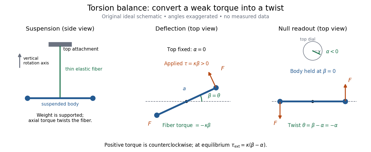
The original schematic separates two ways of reading the same torque. In deflection operation the top attachment stays fixed and the body rotates. In null operation the experimenter rotates the top attachment by $\alpha$ while returning the body's laboratory angle $\beta$ to its original value. If the initially untwisted configuration has $\alpha =\beta =0$, the fiber twist is $\theta =\beta -\alpha$, not $\beta$ alone. ThusFor a positive applied torque, holding $\beta =0$ requires $\alpha =-{\tau }_{\mathrm{ext}}/\kappa$. Keeping the body at the same angle keeps the lever arm and source geometry fixed, making comparison of different applied forces easier. Either readout still requires a calibrated torsion constant and a stable reference orientation.

An illustrative calculation shows the amplification: with $a=0.050\mathrm{m}$, $F=2.0\times 10^{-9}\mathrm{N}$, and $\kappa =1.0\times 10^{-8}\mathrm{N}m/rad$, the applied torque is $1.0\times 10^{-10}\mathrm{N}\mathrm{m}$ and the equilibrium twist is $0.010\mathrm{rad}\simeq 0.573^{\circ }$. These are stipulated values, not measured data. Reducing the torsion constant tenfold increases this twist tenfold, provided the fiber remains in its calibrated linear elasticity range. The cost is a slower response, explained by the oscillation period in torsion constant.

A concrete laboratory experiment is PASCO's Coulomb balance: level its counterbalanced rod, discharge both conducting spheres, and set the unloaded zero. Charge the spheres at maximum separation; switch off the charging supply. Move the second sphere to a known center separation $R$, then turn the suspension dial until the rod returns to its index mark. Record the dial change and $R$, recharge, and repeat at several separations. The manual recommends a draft-free room, clean insulating supports, and recharging before each reading: leakage, especially in humid conditions, otherwise changes the electric charges during the sequence. At close separations the conducting spheres redistribute charge, so the point charge approximation needs correction. ^[ref]

For constant electric charges and a fixed perpendicular lever arm, the Coulomb's law prediction is $|\theta |\propto R^{-2}$. Plotting the logarithm of twist magnitude against the logarithm of separation gives $\log |\theta |=\text{constant}-2\log R$, so the predicted slope is $-2$. Absolute force measurement additionally needs the torsion constant; comparing ratios can eliminate it if it remains stable. Repeating a reference separation between other settings distinguishes a separation effect from a changing signal. A declining reading at the reference separation would invalidate the assumption of unchanged electric charges, even if a distance plot looks smooth.

The historical electrical example is Coulomb's first memoir of 1785. His apparatus enclosed a suspended needle with a small ball and a second ball; an adjustable head twisted the suspension. After charging the balls by contact, he reported angular separations $36^{\circ }$, $18^{\circ }$, and $8.5^{\circ }$ with head settings $0^{\circ }$, $126^{\circ }$, and $567^{\circ }$. The total twists were approximately $36^{\circ }$, $144^{\circ }$, and $576^{\circ }$: fourfold restoring torque accompanied approximately halved separation. These are his reported observations, not data from our diagrams. ^[ref] A precise reconstruction must use center distances and the changing lever arm, rather than identify angular separation exactly with distance; Alberto A. Martínez's replication explicitly analyzes that geometry. ^[ref]

Sensitivity also exposes changes of the apparatus itself. Fleischer and colleagues' cryogenic torsion balance used a temperature-controlled enclosure to reduce vacuum-vessel top-plate temperature fluctuations to approximately $\pm 0.01\mathrm{K}$, limiting changes in suspension geometry from thermal expansion. They used a mild bake-out near $40^{\circ }\mathrm{C}$ to speed initial fiber relaxation and reduce slow zero motion. Their optical readout compared the pendulum mirror with an internal reference mirror to reject shared optical motion. Room-temperature thermal radiation entering through the optical opening heated the pendulum; a cold filter reduced that load. The authors could not directly measure the pendulum's temperature without disturbing it, and explicitly distinguished the cold shield's temperature from the body's. Cooling therefore requires checking the actual noise and thermal environment, rather than assuming that the fiber and body share the shield's temperature. ^[ref]

A useful control strategy is to record unloaded readings and temperature before and after each signal sequence, recalibrate the torsion constant under the same conditions, and compare forward and reverse settings. The algebra of torsion balance zero drift shows precisely which offsets such comparisons can cancel. A fine angular scale alone does not establish a small measurement error.

Tristan Guillot developed analytic radiative-equilibrium models for irradiated planetary atmospheres. They connect incoming stellar radiation and outgoing thermal radiation with a temperature-pressure structure, making assumptions about opacity and irradiation explicit.^[ref]

Anisotropic thermal radiation produces recoil that changes the semi-major axis of a rotating solid body. Finite thermal inertia provides the temperature lag. Large bodies have small acceleration per unit mass, while very small bodies become nearly isothermal. The Yarkovsky effect can supply bodies to dynamical escape regions.

Consider an idealized planet that is a sphere of radius $R$, illuminated by parallel sunlight of irradiance $S$, measured on a plane perpendicular to the rays. Its intercepting projected area is $\pi R^2$, whereas its total surface area is $4\pi R^2$. Therefore the incoming power averaged per unit total surface area iswhere $\alpha$ is the broadband Bond albedo. The factor four is a sphere geometry result, not an atmospheric transmission factor. Local sunlight still varies over the illuminated hemisphere and vanishes on the dark side.

Now stipulate a single spatially uniform temperature $T$, no atmosphere, no internal heating, and emissivity one for outgoing thermal radiation. This is a thermal blackbody model using the Stefan–Boltzmann law; the prescribed solar-band reflection is treated separately, so the body is not a perfect absorber at all wavelengths. Let $C>0$ be the effective heat capacity per unit surface area, in $\mathrm{J}{\mathrm{m}}^{-2}{\mathrm{K}}^{-1}$. Conservation of energy gives the ordinary differential equationHere $F$ is net heating per unit surface area, in $\mathrm{W}{\mathrm{m}}^{-2}$, and $\sigma$ is the Stefan-Boltzmann constant. Use $\sigma =5.670374419\times 10^{-8}\mathrm{W}{\mathrm{m}}^{-2}{\mathrm{K}}^{-4}$, rounded from the exact constant reported by NIST. ^[ref] The uniform temperature is a model assumption: generally the surface average of $T^4$ differs from the fourth power of the surface-average temperature.

For fixed Bond albedo $\alpha$, radiative equilibrium requires $F(T_{\ast })=0$, givingWith the illustrative solar constant $S=1360\mathrm{W}{\mathrm{m}}^{-2}$, the global incoming average is $340\mathrm{W}{\mathrm{m}}^{-2}$:

Doubling albedo here lowers the equilibrium temperature by $33.231\mathrm{K}$, rather than halving it: the absorbed fraction changes from $0.7$ to $0.4$, and thermal radiation scales as $T^4$. These stipulated Bond albedos are whole-planet examples, not measurements of bare water and ice. The model predicts neither Earth's modern surface temperature nor its response to actual climate change; it omits the greenhouse effect, spatial heat transfer and seasons.

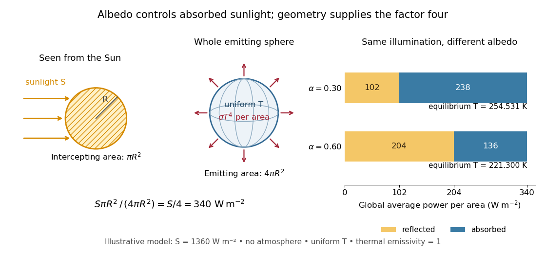
Each fixed-albedo equilibrium is a stable equilibrium: for $T_{\ast }>0$, the derivative is $F^{\prime }(T_{\ast })=-4\sigma T_{\ast }^3<0$. A small temperature increase produces net cooling, and a small decrease produces net heating. This is the simplest expression of the stabilizing Planck feedback. Allowing albedo to fall with temperature adds a competing term, as in ice-ocean albedo feedback.