Thermocouple reference junction ( $T_{c}$ )

The thermocouple reference junction is the connection region where the two thermoelements meet the measurement leads. In ordinary copper-lead wiring there are two material transitions, A–Cu and B–Cu, rather than a second welded A–B junction. They must have a common known temperature

T_{c}

for the simple expression

E (T_{h}, T_{c})

to apply. An ice-water heat bath can establish a nominal

0^{\circ} C

reference; cold-junction compensation instead measures

T_{c}

locally. The word “cold” describes the reference role and imposes no requirement that

T_{c} < T_{h}

Table of contents
- Isothermal terminal block Thermocouple reference junction
- Cold-junction compensation Thermocouple reference junction

Isothermal terminal block

 0  0

An isothermal terminal block keeps the two reference transitions and the reference thermometer at approximately the same temperature, while maintaining electrical insulation between the terminals. Thermal contact is required; an electrical short between A and B would bypass the signal. Merely using copper does not eliminate the Seebeck effect in the meter leads. If both homogeneous copper leads start at

T_{c}

and end at a common meter-input temperature

T_{m}

, their contributions have equal magnitude and opposite sign around the measurement path:

\int_{T_{c}}^{T_{m}} S_{Cu} (T) d T - \int_{T_{c}}^{T_{m}} S_{Cu} (T) d T = 0.

(1)

This cancellation uses matched endpoint temperatures and homogeneous lead material, rather than

S_{Cu} = 0

. A temperature gradient along each lead is allowed under these assumptions. If the two transitions are at different temperatures, one measured

T_{c}

cannot generally correct both; unmatched connectors or wire inhomogeneity can introduce additional electromotive forces. The FP-TC-120 documentation explicitly locates the reference sensing in the terminal base or connector block and specifies isothermal versions of these assemblies.^[ref]

Cold-junction compensation

 0  0

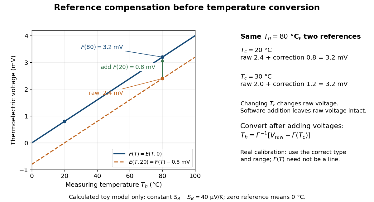
Cold-junction compensation converts a reading with reference temperature

T_{c}

into the equivalent reading for a chosen standard reference. Define the thermocouple reference function

F (T) = E (T, 0)

, where

0

means

0^{\circ} C

, not absolute zero. Additivity of the definite integral gives

E (T_{h}, T_{c}) = F (T_{h}) - F (T_{c}), F (T_{h}) = V_{raw} + F (T_{c}), T_{h} = F^{- 1} (V_{raw} + F (T_{c})) .

(1)

The final inverse function requires a suitable one-to-one calibration interval. A terminal thermometer supplies

T_{c}

independently; the raw thermocouple electric potential difference supplies only the difference of the two reference-function values. In general, first converting

V_{raw}

to a temperature and then adding

T_{c}

is wrong, because the thermocouple reference function need not be linear. The SCC-TC manual explicitly adds the reference-equivalent voltage before its final voltage-to-temperature conversion.^[ref]

For a stipulated model only, take

S_{A} - S_{B} = 40 μ V/K

throughout the interval. No actual material pair is assigned this constant. Because degree Celsius differences have the same numerical size as kelvin differences,

T_{h} = 80^{\circ} C, T_{c} = 20^{\circ} C ⟹ V_{raw} = (40 μ V/K) (60 K) = 2.4 mV .

(2)

In this model

F (20) = 0.8 mV

and

F (80) = 3.2 mV

. Adding the

0.8 mV

correction produces

3.2 mV

, whose inverse calibration gives

80^{\circ} C

. Applying the zero-reference calibration directly to

2.4 mV

would instead display

60^{\circ} C

Now physically change only the reference temperature to

30^{\circ} C

, leaving the measuring junction at

80^{\circ} C

. The raw reading becomes

2.0 mV

; the correction becomes

F (30) = 1.2 mV

, so the corrected total stays

3.2 mV

. Physically changing the reference changes the measured electric potential difference. Adding a software correction changes its interpretation and leaves the raw reading intact. If the actual reference is

30^{\circ} C

but the software still assumes

20^{\circ} C

, this model displays

70^{\circ} C

Figure 1.
Adding the reference-equivalent voltage before inverting the thermocouple reference function
. Calculated constant-Seebeck coefficient-difference example only. The zero-reference line $F (T) = E (T, 0)$ and the $20^{\circ} C$ raw-reading line differ by $F (20) = 0.8 mV$ . At $T_{h} = 80^{\circ} C$ , adding that correction takes $2.4$ to $3.2 mV$ . Changing the reference to $30^{\circ} C$ changes the raw reading and the correction in opposite directions. Real calibration curves need not be straight. **Details**.

An actual implementation in FP-TC-120 and cFP-TC-120 Operating Instructions by National Instruments (p. 7, Cold-Junction Compensation) uses terminal-mounted temperature sensors, reports their reading as “CJ Temperature”, and enables compensation in temperature mode but not voltage mode. This makes the distinction between a raw voltage readout and a compensated temperature readout observable. The specified reference-sensor range also produces an out-of-range indication: a calculated number outside a supported range is not a validated measurement.^[ref]