Thermocouple

A thermocouple uses two different electrical conductors and the Seebeck effect to infer a measuring-junction temperature from a voltage and a known reference temperature. The reference material and the reference temperature are distinct choices: B specifies the comparison Seebeck coefficient, while $T_c$ specifies the lower limit of the integral. The two-material experiment in Seebeck effect gives the geometry, sign convention, and calibration limitations.

The useful measurement is a pair: the raw terminal electric potential difference and the thermocouple reference junction temperature. For the A-positive terminal order and homogeneous-wire assumptions of Seebeck effect, write the open-circuit electromotive force asHere $T_h$ is the thermocouple measuring junction temperature and $T_c$ is the common temperature of the reference connections. The subscript $h$ names the measuring end; it need not be hotter. A voltmeter senses the complete connected thermoelectric path through the wires and its leads, in the electrochemical potential convention already described under Seebeck effect. It does not measure an absolute temperature, the individual Seebeck coefficient of A, or an isolated contact electric potential.

A thermopile connects multiple thermocouples in series to turn a temperature difference into a larger electrical signal. Absorbed thermal radiation can heat its sensing junctions while reference junctions remain cooler; the signal depends on the thermal and optical design.

A thermopile is an array of thermocouples connected as a series circuit with their electromotive forces adding in the chosen terminal order. It measures a collective temperature difference through the Seebeck effect. An open-circuit electric potential difference requires no externally supplied electric current through the array: a high-input-electrical resistance voltmeter reads the signal. The heat that maintains the junction temperature difference still comes from somewhere, such as absorbed electromagnetic radiation.

In a membrane detector, an absorbing film heats the measuring junctions while reference junctions lie on the surrounding support. Actual junction temperatures can differ across the membrane.^[ref] This converts difficult-to-observe heat transfer into an accessible electrical signal; the series connection combines many small contributions without requiring every thermocouple to have a separate meter.

Use the A-positive terminal order of Seebeck effect for each thermocouple. Its thermocouple measuring junction has temperature $T_{h,i}$ and its reference connections have temperature $T_{c,i}$. Define the difference of Seebeck coefficients as ${\alpha }_i(T)=S_{A,i}(T)-S_{B,i}(T)$. Connect the B reference end of one thermocouple to the A reference end of the next at a common local temperature, so the terminal electric potential differences add:The first A reference terminal is the positive meter input; the final B reference terminal is the negative input. Following this connected path and adding the individual Seebeck effect integrals proves the result. Matched meter leads with common endpoint temperatures cancel as in an isothermal terminal block. The manufacturer's sum formula also allows unequal individual contributions.^[ref]

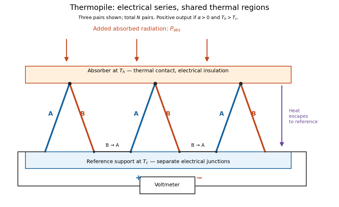
If all pairs share $T_h,T_c$ and the same nearly constant difference $\alpha$ of Seebeck coefficients throughout that temperature interval, thenThis $\alpha$ is the pair's relative Seebeck coefficient, not either material's individual coefficient or a universal device constant. As an original constructed example, choose $N=20$, $\alpha =40\mu \mathrm{V}{\mathrm{K}}^{-1}$ and $\Delta T=5\mathrm{K}$. Each thermocouple contributes $0.20\mathrm{mV}$ andReversing the meter connections changes the sign. Exchanging $T_h$ and $T_c$ reverses the integrals and hence the electromotive force; this reversible sign response does not make a detector with heat conduction a reversible thermodynamic process. Reversing the wiring of one pair instead gives $(N-2)\alpha \Delta T$, because one contribution is subtracted rather than added. For this example the result is $3.6\mathrm{mV}$, and at equal junction temperatures every contribution vanishes.

The open-circuit condition matters. If the array's total electrical resistance is $R_{\mathrm{pile}}$ and the meter input has electrical resistance $R_m$, the elementary voltage divider model gives $V_m=V_{\mathrm{oc}}{R}_m/(R_m+R_{\mathrm{pile}})$. Thus $R_m\gg R_{\mathrm{pile}}$ is needed to suppress voltmeter loading. Appreciable electric current also permits Joule heating and the thermoelectric heat transfer to disturb the assumed junction temperatures.

A thermopile absorber converts incident electromagnetic radiation into heat near the thermocouple measuring junctions. Electrically separate junctions can share its temperature through thermal contact. The reference support provides a path for heat transfer and a comparison temperature; “cold” denotes this reference role, even if it is warmer than the absorber.

Distinguish incident power from absorbed power. A window, the illuminated area, and the absorption of the coating determine their relation. A detector's measured voltage sensitivity can depend on where a small illuminated spot lies.^[ref] The model in thermopile thermal response takes absorbed power as its input, so an optical calibration is a separate step.

A useful original model treats the thermopile absorber as one approximately uniform temperature $T_h(t)$ with heat capacity $C_{\mathrm{th}}$, connected to a fixed reference temperature $T_c$ by thermal conductance $G_{\mathrm{th}}$. Both parameters are positive constants here. Let $P_{\mathrm{abs}}(t)$ be an added absorbed power above the initial background. Linearize the outgoing heat transfer about that background. With $\Delta T=T_h-T_c$ measured from an initial state having $\Delta T=0$, conservation of energy gives the first-order linear differential equationThe left side is the rate of stored energy; the two terms on the right are added power and outgoing heat transfer. The effective thermal conductance can include several paths, rather than just heat conduction along the wires. The model assumes a stable reference, negligible electrical loading, a common absorber temperature, and changes small enough for constant parameters.

For a step from zero to constant $P_0$ at $t=0$, subtract the steady solution $\Delta T_{\infty }=P_0/G_{\mathrm{th}}$. The difference obeys exponential decay, so the initial condition fixesThe time constant has units $(\mathrm{J}{\mathrm{K}}^{-1})/(\mathrm{W}{\mathrm{K}}^{-1})=\mathrm{s}$. With the same constructed $N=20$ and $\alpha =40\mu \mathrm{V}{\mathrm{K}}^{-1}$, choose $C_{\mathrm{th}}=0.02\mathrm{J}{\mathrm{K}}^{-1}$, $G_{\mathrm{th}}=0.01\mathrm{W}{\mathrm{K}}^{-1}$ and $P_0=0.03\mathrm{W}$. ThenAt one time constant, the response is $1-e^{-1}\approx 0.632$ of its final value: $V_{\mathrm{oc}}(2\mathrm{s})\approx 1.52\mathrm{mV}$. Reaching $95\%$ requires $t=-\tau \ln (0.05)\approx 5.99\mathrm{s}$. A voltmeter read too soon therefore underestimates the steady signal even when its electrical calibration is perfect.

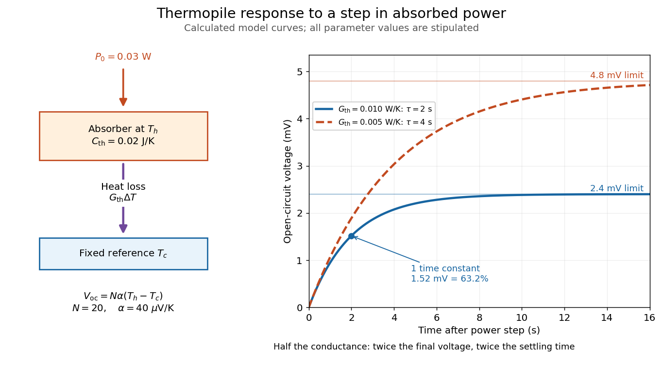
The steady ratio $V_{\infty }/P_0=N\alpha /G_{\mathrm{th}}$ is $0.080\mathrm{V}{\mathrm{W}}^{-1}$ in this constructed model. Halving thermal conductance doubles this ratio but also doubles the time constant if heat capacity stays fixed. Reducing heat capacity alone speeds the response without changing its steady value. Increasing $N$ gives a larger signal only at fixed individual temperature differences: adding legs can also change thermal conductance, heat capacity and electrical resistance. The algebra identifies coupled design choices, rather than predicting a particular manufactured detector.

A finite electrical resistance produces Thermal electrical noise. For nearly uniform absolute temperature $T$ and effective measurement signal bandwidth $B$, its root mean square open-circuit voltage isHere $k_{\mathrm{B}}$ is the Boltzmann constant. Thermal electrical noise in the sensing element is an important contribution, and the signal bandwidth enters its voltage variance.^[ref] If identical pairs have fixed electrical resistance $r$ and fixed $\Delta T$, then $R_{\mathrm{pile}}=Nr$: the signal grows as $N$ while this noise grows as $\sqrt{N}$. The resulting signal-to-noise ratio grows only as $\sqrt{N}$ under those assumptions. Reference temperature drift, environmental electromagnetic radiation, and meter noise remain separate limits; reducing signal bandwidth trades fast information for less integrated electrical noise.

PASCO's documented lamp experiment connects a TD-8553 thermopile sensor to a millivoltmeter and places it level with a lamp filament along a meter stick. Lamp and detector axes are aligned. With the lamp off, readings at several positions establish an average ambient thermal radiation background. With the lamp on at a fixed supply setting, detector readings at different distances are compared after background subtraction. Between readings, a reflective shield prevents the detector warming; its shutter also protects the reference junction when idle. Moving the shutter can move the sensor, so fixed geometry matters. The manual's lamp limits must be followed.^[ref]

This protocol tests whether the background-corrected electric potential difference approximately follows the inverse-square law over a suitable distance range. It is a relative electromagnetic radiation measurement; those readings alone do not calibrate absorbed power in watts. The manual treats the filament as an approximate point source.^[ref]

For an absolute calibration, independently known absorbed power and a monitored reference temperature would be needed. A useful additional control is to repeat a fixed detector position before and after a distance sweep: disagreement reveals possible drift. These additions test the measurement chain rather than assuming that background subtraction fixes every error. A finite source, changing illuminated area, reflections, changing reference temperature, and insufficient settling can alter the measured dependence. In particular, the time constant in thermopile thermal response explains why a quick reading and a settled reading may differ. The detector infers its own absorber temperature difference; inferring the source's temperature additionally requires its emissivity, optical geometry and an appropriate thermal radiation model.

The thermocouple measuring junction joins A and B at the location whose temperature is to be inferred. Its own temperature is what the electrical measurement estimates. To infer a surrounding object's temperature, the junction must approach thermal equilibrium with that object: insufficient immersion, heat conduction along the wires, or a changing environment can keep the junction at another temperature. A stable electrical display alone does not establish that this thermal condition holds. The two-heat bath procedure and terminal-reversal controls under Seebeck effect provide the starting experiment; the practical issue here is the reference and conversion chain.

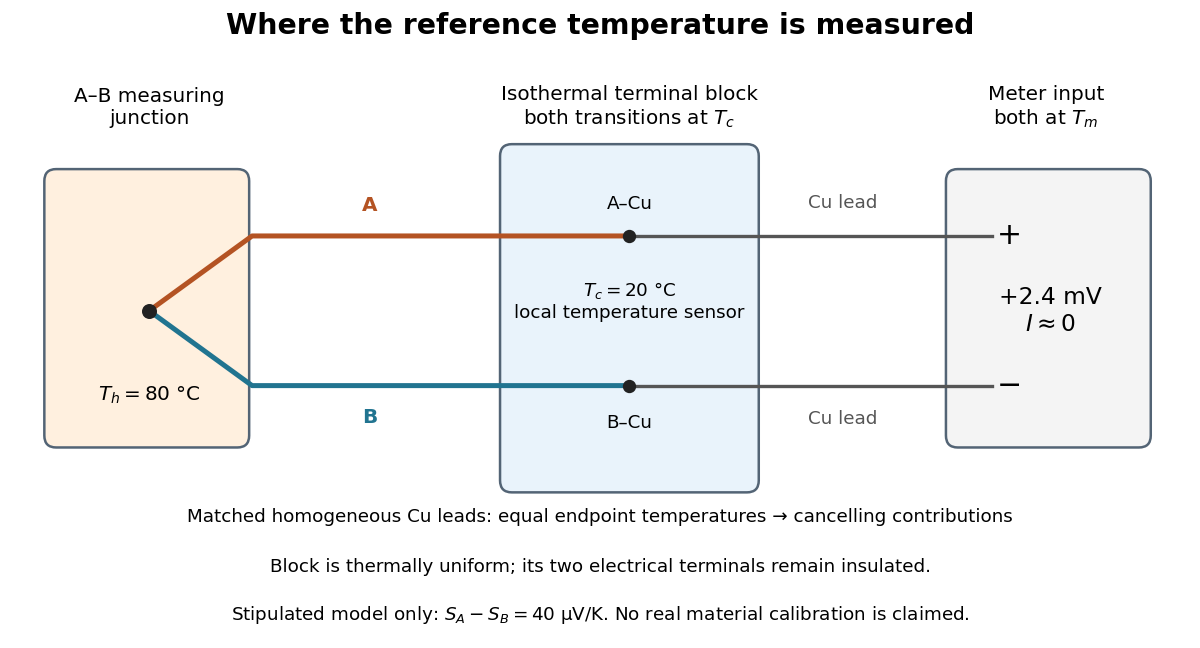
The thermocouple reference junction is the connection region where the two thermoelements meet the measurement leads. In ordinary copper-lead wiring there are two material transitions, A–Cu and B–Cu, rather than a second welded A–B junction. They must have a common known temperature $T_c$ for the simple expression $E(T_h,T_c)$ to apply. An ice-water heat bath can establish a nominal $0{}^{\circ }\mathrm{C}$ reference; cold-junction compensation instead measures $T_c$ locally. The word “cold” describes the reference role and imposes no requirement that $T_c<T_h$.

An isothermal terminal block keeps the two reference transitions and the reference thermometer at approximately the same temperature, while maintaining electrical insulation between the terminals. Thermal contact is required; an electrical short between A and B would bypass the signal. Merely using copper does not eliminate the Seebeck effect in the meter leads. If both homogeneous copper leads start at $T_c$ and end at a common meter-input temperature $T_m$, their contributions have equal magnitude and opposite sign around the measurement path:This cancellation uses matched endpoint temperatures and homogeneous lead material, rather than $S_{\mathrm{Cu}}=0$. A temperature gradient along each lead is allowed under these assumptions. If the two transitions are at different temperatures, one measured $T_c$ cannot generally correct both; unmatched connectors or wire inhomogeneity can introduce additional electromotive forces. The FP-TC-120 documentation explicitly locates the reference sensing in the terminal base or connector block and specifies isothermal versions of these assemblies.^[ref]

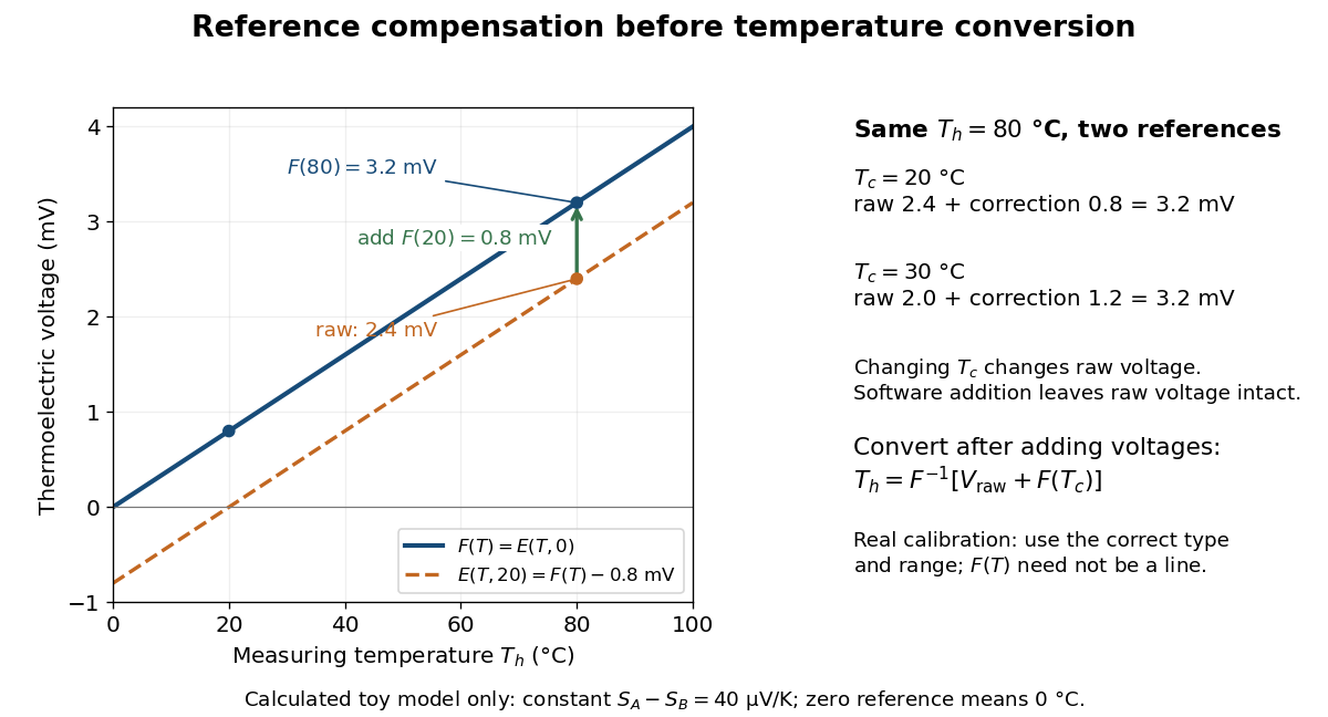
Cold-junction compensation converts a reading with reference temperature $T_c$ into the equivalent reading for a chosen standard reference. Define the thermocouple reference function $F(T)=E(T,0)$, where $0$ means $0{}^{\circ }\mathrm{C}$, not absolute zero. Additivity of the definite integral givesThe final inverse function requires a suitable one-to-one calibration interval. A terminal thermometer supplies $T_c$ independently; the raw thermocouple electric potential difference supplies only the difference of the two reference-function values. In general, first converting $V_{\mathrm{raw}}$ to a temperature and then adding $T_c$ is wrong, because the thermocouple reference function need not be linear. The SCC-TC manual explicitly adds the reference-equivalent voltage before its final voltage-to-temperature conversion.^[ref]

For a stipulated model only, take $S_A-S_B=40\mu V/K$ throughout the interval. No actual material pair is assigned this constant. Because degree Celsius differences have the same numerical size as kelvin differences,In this model $F(20)=0.8\mathrm{mV}$ and $F(80)=3.2\mathrm{mV}$. Adding the $0.8\mathrm{mV}$ correction produces $3.2\mathrm{mV}$, whose inverse calibration gives $80{}^{\circ }\mathrm{C}$. Applying the zero-reference calibration directly to $2.4\mathrm{mV}$ would instead display $60{}^{\circ }\mathrm{C}$.

Now physically change only the reference temperature to $30{}^{\circ }\mathrm{C}$, leaving the measuring junction at $80{}^{\circ }\mathrm{C}$. The raw reading becomes $2.0\mathrm{mV}$; the correction becomes $F(30)=1.2\mathrm{mV}$, so the corrected total stays $3.2\mathrm{mV}$. Physically changing the reference changes the measured electric potential difference. Adding a software correction changes its interpretation and leaves the raw reading intact. If the actual reference is $30{}^{\circ }\mathrm{C}$ but the software still assumes $20{}^{\circ }\mathrm{C}$, this model displays $70{}^{\circ }\mathrm{C}$.

An actual implementation in FP-TC-120 and cFP-TC-120 Operating Instructions by National Instruments (p. 7, Cold-Junction Compensation) uses terminal-mounted temperature sensors, reports their reading as “CJ Temperature”, and enables compensation in temperature mode but not voltage mode. This makes the distinction between a raw voltage readout and a compensated temperature readout observable. The specified reference-sensor range also produces an out-of-range indication: a calculated number outside a supported range is not a validated measurement.^[ref]

Thermocouple voltage calibration relates an actual assembled sensor's electromotive force to independently established junction temperatures. It must be distinguished from selecting a nominal letter-type conversion curve. In Thermocouples Calibrations Services by National Institute of Standards and Technology (opening method description and bath-calibration table), NIST describes comparison with a maintained reference thermocouple, comparison with a standard platinum resistance thermometer in controlled heat baths, and fixed-point calibration at the freezing points of zinc, aluminum, silver and gold on the International Temperature Scale of 1990. These are independent thermal references, unlike a test that checks only a voltage-input circuit.^[ref]

For a concrete electrical check, the SCC-TC guide describes shorting the input after 30 minutes of powered operation and adjusting its offset to a zero-voltage readout. Its separate calibrator procedure requires equal connection temperatures at the calibrator and module, measures the supplied voltage, converts it to temperature, and compares with the calibrator setting. Such an injected-signal test checks the readout chain; it does not expose a real measuring junction to an independently known bath temperature.^[ref]

Useful additional checks follow from the model: log the raw voltage, the reference temperature, and the final inferred temperature separately; hold $T_h$ stable while changing $T_c$ and test whether cold-junction compensation preserves the inferred $T_h$; compare against an independent thermometer at several stable heat bath settings. Check immersion and repeatability instead of assuming a steady display establishes thermal equilibrium. These are proposed diagnostic checks, not new experimental results. The equal-temperature and polarity controls are already described under Seebeck effect.

Limits arise separately from the thermocouple reference function, sensor-wire changes, thermal contact, terminal temperature differences, and the voltage-input circuit. In particular, the SCC-TC guide warns of connector-to-module temperature gradients and voltage drops caused by the fault-detection electric current flowing through lead electrical resistance.^[ref] A fitted curve or compensation algorithm cannot make all these errors vanish. No single accuracy is assigned to every thermocouple.

A thermocouple reference function gives the nominal thermoelectric electromotive force versus temperature for a specified material pair and reference temperature, conventionally $0{}^{\circ }\mathrm{C}$. Real Seebeck coefficients vary with temperature, sois generally nonconstant. A lookup calibration can use interpolation between tabulated values; a fitted calibration can use polynomials over stated intervals. Use the correct material type, units, reference and validity interval in both the forward and inverse conversions. The FP-TC-120 manual specifically requires the channel's thermocouple type to be configured and describes its use of NIST-175 reference characteristics.^[ref] A nominal reference curve is not evidence that an aged or inhomogeneous wire still follows it.

A local error estimate explains why the reference thermometer matters. If $\delta V$ is an additive voltage error and $\delta T_c$ is the error in the supplied reference temperature, differentiation of the compensation equation gives, for $F^{\prime }(T_h)\ne 0$,A small slope $F^{\prime }(T_h)$ magnifies voltage errors. In the stipulated $40\mu V/K$ model, a $40\mu \mathrm{V}$ offset gives a $1\mathrm{K}$ inferred-temperature error, and a $1\mathrm{K}$ reference error gives a $1\mathrm{K}$ inferred-temperature error. These are sensitivities of the chosen model, not universal performance figures for real sensors.