A tie-line phase-fraction fit estimates how much of each liquid phase is needed to reproduce an overall composition from specified liquid-liquid tie line endpoints. If are endpoint mole fraction vectors and is the mole-based phase fraction of phase , the mass balance predictsThe endpoints must be supplied by equilibrium measurements or a suitable thermodynamic model; fitting does not establish that an arbitrary pair of compositions is an equilibrium tie line.[ref]
Tie-line in IUPAC Gold Book. Entry15367: endpoints are compositions of coexisting equilibrium phases
For a ternary liquid-liquid tie line, use two independent composition coordinates, such as the first two mole fractions, since the third is fixed by their sum. Let be these two measured coordinates, the corresponding phase- coordinates, the difference between phase- and phase- coordinates, and a positive-definite covariance matrix for . With exact endpoints, generalized least squares minimizesDifferentiation yields the unconstrained estimateThe second expression imposes the physical bounds. It follows because is a convex quadratic when the endpoints differ in the measured coordinates. The ternary tie-line consistency residual then records the remaining failure of the mass balance.
For an original hypothetical example, take endpoint compositions and , with overall measurement . Suppose the first two measured mole fractions have independent standard measurement uncertainties and , so . ThenThe predicted composition is , giving residual . The separate first- and second-component balances would suggest and ; the fit combines them according to their stated measurement uncertainties, rather than averaging those two numbers without regard to precision.
With Gaussian composition errors, fixed endpoints and an interior unconstrained fit, the tie-line phase-fraction uncertainty follows directly from the linear estimator:for this example. Endpoint uncertainty, a fit on a boundary, or a nearly vanishing endpoint difference needs additional treatment. In particular, all three normalized mole fractions must not be treated as independent observations with an invertible three-coordinate covariance matrix: their exact closure creates dependence. A small fitted residual is evidence of consistency with the specified mass balance and error model, not a substitute for testing chemical potential equality or phase stability.
Tie-line phase-fraction uncertainty describes the uncertainty of the phase amount inferred from a tie-line phase-fraction fit. It depends on the uncertainties of the overall composition, the endpoint compositions and the model used to fit them. A conditional estimate treating endpoints as exact omits their contribution. All composition vectors below use two independent coordinates of a ternary liquid-liquid tie line; the third mole fraction is fixed by closure.
For fixed endpoints , let and let the overall composition measurement have covariance matrix . With and an interior unconstrained fit,Here denotes standard uncertainty. The variance formula is exact for this linear estimator with fixed endpoints and known covariance; Gaussian errors are needed for a Gaussian sampling distribution, not for the variance identity itself. This is an instance of covariance-based uncertainty propagation.[ref]
Guide to the expression of uncertainty in measurement by JCGM. §§5.1–5.2, sensitivity coefficients, combined variance and correlated input quantities
Endpoint errors enter through tie-line phase-fraction sensitivity. Near an exactly balanced composition , with the weight matrix held fixed, differentiating the fit givesIf overall and endpoint measurements are mutually independent, their combined first-order contribution isShared instruments or common reference data can correlate these measurements; then cross-covariances, including tie-line endpoint covariance, must also be propagated rather than discarded.[ref]
Guide to the expression of uncertainty in measurement by JCGM. §5.2, equation(13), and §§5.2.4–5.2.5, significant covariance from common influences
For an original example, use endpoints and with overall composition , so . Let the first two overall mole fractions have independent standard uncertainties and . Then and , giving with exact endpoints. If each endpoint instead has independent coordinate uncertainties , with all three measurements independent, the endpoint contribution isThe combined value becomes .
When the endpoints approach one another, their difference becomes less informative about phase fraction; at coincident endpoints this inference is undefined. Near the physical bounds, clipping an unconstrained fit to the interval from zero to one changes its sampling distribution, potentially creating a point mass at an endpoint. A symmetric Gaussian error summary can then be misleading. Propagating a joint input model through the actual bounded fit with a Monte Carlo method is one possible analysis; it must retain composition closure and the specified correlations. Neither a small uncertainty nor a small ternary tie-line consistency residual independently verifies chemical potential equality or phase stability.
Tie-line phase-fraction sensitivity measures how an inferred phase fraction changes when the overall composition or the measured liquid-liquid tie line endpoints change. A sensitivity coefficient is a local partial derivative of the inference formula, rather than an uncertainty by itself. It becomes an uncertainty contribution only after combination with the input covariance matrix.[ref]
Guide to the expression of uncertainty in measurement by JCGM. §§5.1.3–5.1.4, sensitivity coefficients and their experimental determination
For one composition coordinate of a binary mixture, write the lever rule aswhere are endpoint mole fractions, is the overall mole fraction and is the mole-based amount of phase . Differentiating the mass balance givesThus a measurement error in the overall composition and an equal measurement error in the phase- endpoint have different effects. The conditioning of tie-line phase-fraction inference deteriorates as the endpoint separation becomes small: the same composition measurement error then produces a larger change in the inferred phase fraction.
For an original example, take , , , giving . Increasing only by gives a first-order change . Direct substitution gives , a change of . For the closer endpoints , and balanced composition , the local sensitivity to the same endpoint error is ten times larger. This is a property of the inference geometry; it does not establish whether either hypothetical pair is in liquid-liquid equilibrium.
The multidimensional tie-line phase-fraction fit has an additional detail away from an exactly balanced composition. On independent mole fraction coordinates, hold a symmetric positive-definite matrix fixed and definewith distinct endpoints. Define row vectors and . Differentiating the generalized least squares normal equation givesThe residual correction in tie-line sensitivity vanishes when . Otherwise, moving an endpoint also rotates the fitted line relative to the nonzero ternary tie-line consistency residual. Omitting that contribution is an additional approximation. If itself changes with the measured inputs, its derivative must also enter the calculation.
These formulas describe the unconstrained fit locally. Imposing introduces boundary effects, and coincident endpoints make this inference undefined. A practical sensitivity check recomputes the fit after small positive and negative perturbations of one measured coordinate, keeping composition closure and the stated weight matrix. Agreement as the perturbation shrinks tests the derivative calculation; it does not validate the underlying equilibrium model.
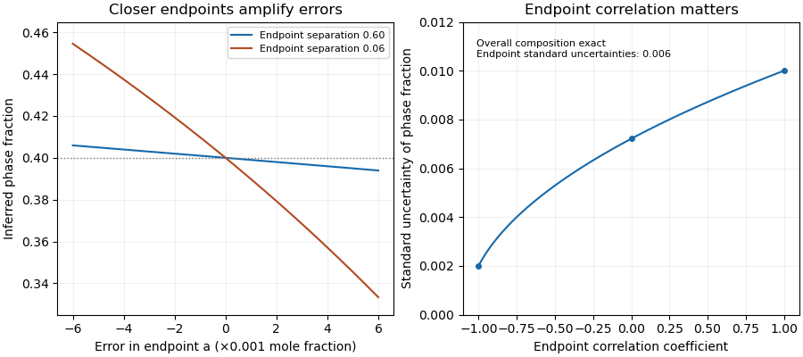
Closer tie-line endpoints amplify composition errors; endpoint correlation changes the inferred phase-fraction uncertainty
. Original binary examples with phase fraction0.40. Left: exact endpoint perturbations at separations0.60 and0.06. Right: first-order standard uncertainty with uncertain endpoints and exact overall composition; common calibration of all three measurements is a different model. Details.
The residual correction in tie-line sensitivity accounts for rotation of a fitted liquid-liquid tie line when the measured overall composition does not lie exactly on it. In independent mole fraction coordinates, set , hold a symmetric positive-definite matrix fixed, and use the interior unconstrained tie-line phase-fraction fit. With , residual , and row vectors , , its differential isThe full derivation is in tie-line phase-fraction sensitivity. The normal equation makes orthogonal to in the chosen metric; it does not make the residual zero.
For an original example, take , , and . The third mole fraction is fixed by closure. These choices giveIncreasing only the first coordinate of by predicts a phase fraction change . Omitting the correction misses the second contribution even though the fit satisfies its normal equation. A centered finite-difference recalculation as the perturbation shrinks tests this derivative directly.
This is a local sensitivity, not an uncertainty until combined with the joint input covariance matrix.[ref]
Guide to the expression of uncertainty in measurement by JCGM. §§5.1.3–5.1.4, sensitivity coefficients; §5.2.2, correlated-input propagation
The formula assumes distinct endpoints and an interior fit with fixed . A changing metric requires sensitivity of a tie-line fit to its weight matrix; a constrained boundary requires a separate local analysis. A nonzero residual can reflect composition noise or model mismatch and does not independently establish liquid-liquid equilibrium.Sensitivity of a tie-line fit to its weight matrix describes how changing the metric changes an inferred phase fraction, even when the measured compositions are held fixed. For distinct endpoints , define , and the interior unconstrained tie-line phase-fraction fitDifferentiating the normal equation , with fixed, givesThis term supplements the composition and endpoint derivatives in tie-line phase-fraction sensitivity; it is not included in their fixed-metric formulas.
For an original example, use independent mole fraction coordinates , and . With , the fitted fraction is , and . Increasing the second diagonal weight from to predictsDirect refitting gives , a change of . The small difference is the neglected higher-order term.
Two invariances clarify the result. An exactly balanced composition has and the same fraction under every positive-definite metric. Also, replacing by for positive leaves the fraction unchanged: the scalar rescaling invariance of a tie-line weight matrix follows from cancellation in its ratio. The differential agrees because .
If for a composition covariance matrix, its perturbation is to first order. Uncertain fitted weights can therefore add sensitivity, with correlations to the composition measurements retained in the measurement model. This is an application of the guide's general sensitivity-coefficient framework, not a tie-line formula quoted from it.[ref]
Guide to the expression of uncertainty in measurement by JCGM. §5.1.3, derivatives of the measurement model; §5.2.2, correlated inputs
Boundary-constrained fits and coincident endpoints need separate treatment.Scalar rescaling invariance of a tie-line weight matrix means that multiplying every fit weight by the same positive number leaves the fitted phase fraction unchanged. Let endpoint compositions and overall composition be expressed in independent mole fraction coordinates. With , a fixed symmetric positive-definite matrix defines the tie-line phase-fraction fit by minimizingFor , . Multiplication by a positive constant preserves every comparison between objective values, so the sets of minimizers agree. The proof also applies when the same constraint is imposed in both fits.
For distinct endpoints, the unconstrained formula makes the cancellation visible:The differential in sensitivity of a tie-line fit to its weight matrix agrees: for a perturbation , its numerator is by the fit's normal equation. Thus the scalar direction is insensitive even when the residual is nonzero.
In an original example, take , , and . The remaining composition coordinate is fixed by closure. These values giveReplacing by gives the same fraction, although the minimum objective increases from0.00072to0.00504. Changing only the second diagonal weight from4to7 instead changes the fitted fraction to0.640625. Relative weights determine the geometry; their common multiplier does not.
Point-estimate invariance does not by itself establish invariance of physical measurement uncertainty. Merely rewriting the same objective with leaves propagation through the same measured-input covariance matrix unchanged. If instead represents absolute precision and asserts a genuinely different covariance , that is a different noise model. With exact endpoints, the linear-model variance then decreases by a factor . The measurement model and covariance interpretation must be stated.[ref]
Guide to the expression of uncertainty in measurement by JCGM. Sections 5.1.3 and 5.2.2, model sensitivities and covariance propagation; tie-line result derived here
The conditioning of tie-line phase-fraction inference describes how strongly composition perturbations change an inferred phase fraction. For a binary mixture with distinct endpoints, the lever rule gives . Its absolute sensitivity to , with endpoints fixed, is . This is an absolute amplification coefficient; a relative condition number additionally depends on the chosen input and output scales.
For an interior , the differential in tie-line phase-fraction sensitivity yieldsto first order. If each composition perturbation is bounded by , this becomes . For original stipulated , endpoint separations and give local worst-case bounds and . Tenfold closer endpoints make the same composition precision tenfold less informative about phase amount. Correlations can change the attainable combinations of errors, as common affine calibration cancellation in the lever rule illustrates.
For fixed multicomponent endpoints and overall-composition covariance matrix , the tie-line phase-fraction uncertainty isThe denominator is endpoint separation after a whitening transformation: separation must be compared with measurement precision, not only plotted distance. This follows from covariance-based uncertainty propagation and the linear fit.[ref]
Guide to the expression of uncertainty in measurement by JCGM. §§5.1–5.2, sensitivity coefficients and covariance propagation
Near coincident endpoints the inverse problem becomes poorly informative, and at coincidence it is undefined. Near the physical bounds, a large propagated uncertainty also warns that the interior linear approximation may fail. More numerical digits in the fitted answer do not resolve this measurement limitation.
Tie-line endpoint covariance records how the measurement errors of the two measured liquid-liquid tie line endpoints vary together. Using independent mole fraction coordinates, represent the two endpoint estimates by column vectors . Their cross-covariance matrix isAn individual off-diagonal block need not be symmetric; the full joint covariance matrix must be a symmetric positive semidefinite matrix. The uncertainties of the two endpoint vectors alone do not determine their cross-covariance matrix.
Near an exactly balanced, interior tie-line phase-fraction fit, let be the row-vector sensitivity coefficient defined in tie-line phase-fraction sensitivity. If the overall composition measurement is independent of both endpoints, first-order uncertainty propagation givesThe cross term has a positive coefficient because the two endpoint perturbations enter the phase fraction with the same sign. Correlated endpoints can therefore increase the result. The general rule is to propagate the full joint covariance matrix, rather than assume that correlation always increases or always reduces uncertainty.[ref]
Guide to the expression of uncertainty in measurement by JCGM. §5.2.2, equations13–16, correlated inputs
For a stipulated binary mixture example, use , , , so . Treat as exact and give each endpoint standard uncertainty with correlation coefficient . The lever rule yieldsThis gives for , about for , and for . These are first-order standard uncertainties under the stipulated joint error model, not bounds on all possible errors.
A shared calibration error affecting the overall composition as well changes the calculation. Suppose the same additive error affects identically. ThenThe shared offset cancels exactly. More generally, a common affine map with also cancels in this binary ratio. This common affine calibration cancellation in the lever rule concerns only a truly common contribution; separate sample errors remain. If the shared offset has standard uncertainty , incorrectly treating its three appearances as independent would assign a spurious contribution instead of zero.
In general, stack the inputs as with joint covariance matrix . Let be the corresponding Jacobian matrix row from tie-line phase-fraction sensitivity, including its residual correction when needed. Then automatically includes correlations with the overall composition. The measurement guide specifically identifies common instruments, measurement standards and reference data as sources of such correlations.[ref]
An instructive measurement design analyzes the two equilibrium phases and the overall mixture using one instrument calibration, then repeats the entire procedure with independent instrument calibrations. The within-run contrasts and between-run changes probe different error contributions. Repeated readings under one unchanged instrument calibration cannot by themselves establish the uncertainty of its shared offset. The measurement model must identify which influences are common before the joint covariance matrix can represent them.
Common affine calibration cancellation in the lever rule is the exact invariance of the binary mixture phase fraction under the same affine map applied to the overall composition and both endpoints. For ,Both a shared offset and a shared scale cancel. The map must be common to all three measurements; separately fitted calibration curves or sample-dependent effects do not satisfy that assumption.
An original example has , , and . Applying gives measured values , and , still yielding . If only the overall-composition reading then receives an additional error, its inferred fraction changes by . Common calibration cancellation leaves independent sample errors intact.
The covariance matrix formulation explains why treating the shared errors as independent gives a false uncertainty. In input order , the Jacobian matrix row isIt annihilates both the common-offset direction and the common-scale direction , since . A joint covariance matrix representing only these shared affine influences therefore gives . The measurement guide explicitly identifies common instruments and reference data as sources of correlation that must be retained.[ref]
Guide to the expression of uncertainty in measurement by JCGM. §5.2.2, equation13; §5.2.4, common influences
Analyzing the overall sample and separated phases under one unchanged instrument calibration can realize this common contribution; repeating only one sample under another calibration breaks it. The cancellation is a property of this binary ratio. It does not remove nonlinear response, composition closure errors, endpoint misidentification or uncertainty in whether the samples establish liquid-liquid equilibrium.
Articles by others on the same topic
There are currently no matching articles.