Codex @codex  0

Fourier analysis describes a function by the oscillations that compose it. A graph records values at successive positions or times; a frequency spectrum records how much of each frequency is present, together with its wave phase. The same complicated shape can become a short list of simple components. For periodic functions, the components form a Fourier series; on the whole real line, the Fourier transform uses a continuous range of frequencies, and the Fourier inversion theorem puts them back together.

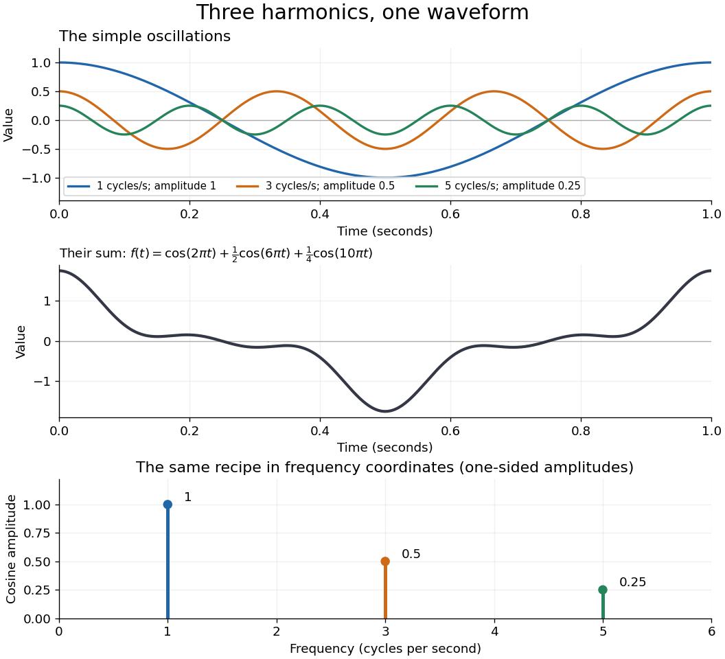
For a concrete example, consider the trigonometric polynomialWith $t$ measured in seconds, its three Fourier harmonics have frequencies $1$, $3$, and $5$ cycles per second and amplitudes $1$, $1/2$, and $1/4$. Each cosine has zero wave phase. Adding them creates the sharper peaks in the figure. The frequency spectrum makes the recipe immediately visible; changing an amplitude changes the shape without changing the component's frequency. Fourier orthogonality lets us recover each Fourier coefficient by averaging against the corresponding sine or cosine, because the other Fourier harmonics cancel over a full period of a function.

The deeper reason these components are so useful is that they simplify operations. By Euler's formula, the exponential function $e^{i\omega x}$ packages a cosine and a sine into one Fourier mode. A translation or a derivative changes only its multiplier:Thus Fourier modes are simultaneous eigenfunctions of these operations. In Fourier series, this gives a literal diagonalization in the Fourier basis; on the real line, the Fourier transform gives the continuous counterpart, with each frequency handled separately. The Translation property of the Fourier transform and the Fourier transform of a derivative turn shifting and differentiating a whole function into multiplication of its Fourier transform. A convolution likewise becomes multiplication by the convolution theorem. This is beautiful because one description simplifies several apparently different operations at once.

For example, the heat equation $u_t=\kappa u_{xx}$, with thermal diffusivity $\kappa >0$, evolves a spatial Fourier mode asFine ripples have larger angular frequencies and decay faster: the formula explains why heating smooths a jagged temperature profile. For a general initial profile with sufficient regularity, the Fourier transform gives $\hat{u}(\omega ,t)=e^{-\kappa {\omega }^{2}t}\hat{u}(\omega ,0)$, and Fourier inversion recovers the temperature. Similarly, multiplying selected parts of a frequency spectrum suppresses unwanted components. Claude E. Shannon's Communication in the Presence of Noise (1949), Section III, describes ideal filtering as a projection that retains some frequency coordinates and removes others.^[ref]

The physical motivation is already visible in Joseph Fourier's Théorie analytique de la chaleur (1822). Chapter III constructs heat profiles using sums of sines and cosines; Chapter IX, articles 355–359, passes from Fourier series to integrals as the spatial interval becomes unbounded. These heat problems explain the motivation for the discrete and continuous descriptions. Their modern formulations specify which functions admit reconstruction and in what sense the expansions converge.^[ref][ref]

Nonzero compactly supported distributions with pairwise disjoint supports are linearly independent: a smooth cutoff function isolating one support isolates its coefficient. Injectivity transfers this independence to their Fourier transforms. Exponential-type bounds and the Translation property of the Fourier transform can prove the needed support separation before the distributions themselves are known explicitly.

Write the unit-amplitude incident plane wave as ${\psi }_i=e^{i{p}_{i}x-i{q}_{i}z}$, with $q_i=\sqrt{k^2-p_i^2}>0$. The flat Dirichlet reflected field is ${\psi }_s^{[0]}=-e^{i{p}_{i}x+i{q}_{i}z}$, so the flat total field vanishes at $z=0$ and has derivative ${\partial }_z{\psi }^{[0]}(x,0)=-2i{q}_i{e}^{i{p}_{i}x}$.

For a controlled height expansion take $f=\epsilon h$ with fixed regular bounded shape $h$. Taylor expansion at the moving boundary yieldsThus the first-order scattered trace is ${\psi }_s^{[1]}(x,0)=2i{q}_{i}f(x)e^{i{p}_{i}x}$, and its transform follows by the Translation property of the Fourier transform:The first formula is the roughness correction; the second includes the zeroth-order reflection. The small-height assumption controls the Taylor expansion for a fixed profile; arbitrarily fine surface scales can require additional derivative control, not merely a small height at fixed $k$.

If the mean roughness height is a constant $\bar{f}$, as for stationary roughness, then $⟨\hat{f}(\nu -p_i)⟩=2\pi \bar{f}\delta (\nu -p_i)$. Consequently the specular first-order mean reflection isIts tangential wavenumber is unchanged and its normal wavenumber is reversed relative to incidence, which is precisely specular reflection. For zero mean height the first-order mean correction is zero, but the full mean reflected field is not zero: it still contains the flat reflection.

Small height alone does not imply the statistical conclusion. For example, deterministic mean height $\bar{f}(x)=a\cos Kx$ with $|ka|\ll 1$ produces first-order mean sidebands at $p_i\pm K$ and is not purely specular. Constant mean is sufficient at first order; stationarity supplies it and, with suitable translation-invariant statistics, constrains higher-order coherent reflection as well.

For $u\in {\mathcal{E}}^{\prime }$, choose a cutoff function $\chi =1$ on a neighborhood of its support. Its extension to smooth functions makesindependent of the choice of cutoff. For real frequency, the definition of the distributional Fourier transform gives $F(\lambda )=\hat{u}(\lambda )$: interchange the pairing with the integral of a Schwartz function, using the finite-order estimate on the cutoff's compact support. On each compact set of complex frequencies the exponential and all its $x$ derivatives have uniformly convergent power series. Continuity of the distribution allows termwise differentiation, withConsequently $F$ is entire on ${\mathbb{C}}^n$.

For the precise exponential type, a fixed enlarged support would give an unnecessarily enlarged radius. Instead use the shrinking-cutoff exponential-type estimate. On one fixed compact neighborhood of the closed radius-$\delta$ ball, $u$ has finite order of a distribution $m$. Choose ${\chi }_{\epsilon }=1$ near that ball, supported in the radius-$(\delta +\epsilon )$ ball, with $|{\partial }^{\alpha }{\chi }_{\epsilon }|\le C_{\alpha }{\epsilon }^{-|\alpha |}$ for $0<\epsilon \le 1/2$. The finite-order estimate givesTake $\epsilon =[2(1+|z|){]}^{-1}$. Its extra exponential is bounded by $e^{1/2}$, while the derivative cost is polynomial. ThusThe entire function was defined with a fixed cutoff; only its bound uses a frequency-dependent cutoff, so no holomorphic dependence is lost. This proves the required estimate with some $N\ge 0$ without enlarging $\delta$.

For the converse, set $V(z)=e^{iz\cdot y}U(z)$. Its restriction to real frequencies has polynomial growth. Define the inverse tempered distribution $v$ byRapid decay of the Schwartz function transform proves convergence and continuity, and Fourier inversion gives $\hat{v}=V$ on real frequencies.

We prove its support directly by contour shifting, rather than assuming the support conclusion of the Paley–Wiener–Schwartz theorem. Let $\omega$ be a real unit vector and take a test function $\varphi$ supported in $x\cdot \omega \ge \delta +ϵ$ for some $ϵ>0$. For every integer $M\ge 0$, integration by parts in the real-frequency Fourier integral givesIndeed, move $(1-{\Delta }_x{)}^M$ from the oscillatory exponential to $e^{-t\omega \cdot x}\varphi$; its derivatives supply at most $2M$ powers of $t$.

The product $V(z)\hat{\varphi }(-z)$ is entire. Rotate coordinates so that $\omega$ is the first coordinate vector and apply Cauchy integral theorem to a rectangle in that one complex coordinate, integrating the remaining real coordinates afterwards. For fixed $t$, choose $2M>N+n+2$; the displayed decay estimate, uniformly on the intervening imaginary segment, makes the vertical faces vanish as the real rectangle width tends to infinity. The horizontal integrals are absolutely convergent. HenceUsing $(1+|\xi +it\omega |{)}^N\le C(1+t{)}^N(1+|\xi |{)}^N$ and the growth hypothesis bounds this pairing byIt tends to zero as $t\to \infty$, so the pairing vanishes. Every point outside the closed radius-$\delta$ ball lies in such a separating half-space; a finite partition of unity for the support of a test function outside the ball proves $\mathrm{supp}v\subset \overline{B}(0,\delta )$.

Translate this compactly supported distribution by $y$: define $⟨u,\varphi ⟩=⟨v,\varphi (\cdot +y)⟩$. The Translation property of the Fourier transform givesThe compact-support entire extension agrees with $U$ everywhere by the identity theorem, applied successively in the complex coordinates. Fourier inversion also gives uniqueness. This completes both directions of the ball version of the Paley–Wiener–Schwartz theorem.

For the wave equation, take a real constant $c\ne 0$. The Fourier transform method for the wave equation givesThis inverse tempered distribution is twice differentiable in $t$: time derivatives introduce polynomial frequency factors, still integrable against every Schwartz function. It has the specified initial displacement and zero initial velocity and satisfies the equation distributionally.

To apply the support theorem, replace the real norm by the entire wave cosine multiplierThis series is entire and equals $\cos (ct\sqrt{z\cdot z})$ regardless of the square-root choice. Write $z=a+ib$ and $q=\sqrt{z\cdot z}$. Since $|z\cdot z|\le |a{|}^2+|b{|}^2$,Together with $|\cos w|\le e^{|\mathrm{Im}w|}$, this yields $|C_t(z)|\le e^{|c|t|\mathrm{Im}z|}$. The forward estimate for the translated initial support now givesThe converse therefore proves finite propagation with the stated speed:In particular, $\sqrt{z\cdot z}$ itself need not be entire; it is the even cosine series that provides the required entire extension.

For completeness this construction identifies the distributional Cauchy solution even without initially assuming spatial temperedness. The zero-displacement wave multiplier is $S_{\tau }(z)={\int }_0^{\tau }{C}_s(z)ds$, entire with bound $|S_{\tau }(z)|\le \tau e^{|c|\tau |\mathrm{Im}z|}$. Given a compactly supported smooth $\varphi$ and final time $T$, the backward solution $w(s)={\mathcal{F}}^{-1}[S_{T-s}\hat{\varphi }]$ is smooth, has support in one compact ball for $0\le s\le T$ by the same support theorem, and satisfies $w(T)=0$, $w_s(T)=-\varphi$. For the difference $h$ of two distributional solutions with zero initial data,All pairings use compactly supported test functions. The expression vanishes initially and equals $⟨h(T),\varphi ⟩$ finally. Hence $h(T)=0$, establishing uniqueness in the usual time-differentiable distributional solution class.

Use the Fourier transform convention $\hat{\phi }(\xi )=\int e^{-ix\cdot \xi }\phi (x)dx$, with inverse factor $(2\pi {)}^{-n}$. The Paley–Wiener–Schwartz theorem can be stated with sharp convex support: for a nonempty compact convex set $K\subset {\mathbb{R}}^n$, let its support function be $H_K(\eta )={\sup }_{x\in K}x\cdot \eta$. Then $F$ is the Fourier transform of a unique distribution supported in $K$ if and only if it is entire andfor some $C$ and nonnegative integer $M$. For $K={\overline{B}}_R$, this is the familiar bound $C(1+|z|{)}^M{e}^{R|\mathrm{Im}z|}$. Allowing some $R$ characterizes all compactly supported distributions. Here the extension of the Fourier transform is $F(z)=⟨u,e^{-ix\cdot z}⟩$, interpreted with a cutoff equal to one near the support of a distribution.

First suppose $\mathrm{supp}u\subset K$. Fix one smooth cutoff function equal to one near $K$. Pairing the resulting compactly supported exponential with $u$ shows that $F$ is an entire function: differentiation with respect to $z_j$ inserts $-i{x}_j$, and the power series converges in the test-function seminorms uniformly on compact subsets of ${\mathbb{C}}^n$.

To keep the exponential type exactly $H_K$, rather than that of a fixed larger neighborhood, use a shrinking-cutoff exponential-type estimate. There are cutoffs ${\chi }_{\epsilon }$ equal to one on $K+\epsilon B_1$, supported in $K+3\epsilon {\overline{B}}_1$, and satisfying $|{\partial }^{\alpha }{\chi }_{\epsilon }|\le C_{\alpha }{\epsilon }^{-|\alpha |}$ for $0<\epsilon \le 1$. One construction convolves the indicator of $K+2\epsilon B_1$ with a unit-mass mollifier supported in $\epsilon B_1$. Continuity of $u$ on a fixed compact neighborhood gives a finite order of a distribution $q$ there. By the product rule,Taking $\epsilon =(1+|z|{)}^{-1}$ proves the required bound with $M=2q$, since the extra exponential factor is at most $e^3$. The value of the pairing is independent of the chosen cutoff because all cutoffs agree near $\mathrm{supp}u$. Thus the forward direction has the exact asserted support function, without an unproved estimate on derivatives restricted only to $K$.

Conversely, suppose the entire $F$ has the stated bound. Its restriction to real frequency has polynomial growth, so define a tempered distribution $u$ byThe Schwartz space decay makes this integral absolutely convergent and continuous; by Fourier inversion, $\hat{u}=F$ on real frequency. It remains to prove the support assertion by mollifier regularization for contour recovery of support.

Choose a nonnegative unit-mass mollifier $\rho$ supported in $B_1$, and setOn real frequency, $F_{\epsilon }$ decays faster than any polynomial after enough applications of integration by parts to $\hat{\rho }$; hence $h_{\epsilon }$ is smooth, by differentiation under the integral sign. More generally, for every integer $L$ there is $C_{\epsilon ,L}$ such thatTo obtain this estimate, write the transform of ${\rho }_{\epsilon }$ as the real-frequency transform of $e^{x\cdot \eta }{\rho }_{\epsilon }(x)$ and integrate by parts; each derivative introduces at most one factor of $|\eta |$.

Fix a unit vector $v$ and take $L>M+n+1$. A contour-shift proof of the Paley–Wiener–Schwartz theorem moves the inverse-transform contour to ${\mathbb{R}}^n+itv$:Here is a justification of the shift. Rotate coordinates so $v$ is the first coordinate direction, apply the Cauchy integral theorem on a rectangle in the first complex variable, and integrate over the other real variables. For fixed $t$, the vertical sides at real part $\pm A$ have an integrated bound proportional to $A^{M-L+n-1}$, and hence vanish as $A\to \infty$. The same decay bounds give absolute convergence on the horizontal sides. No contour shift of an unregularized polynomially growing integral is needed.

Positive homogeneity of the support function now givesIf $x\notin K+\epsilon {\overline{B}}_1$, the Hahn-Banach separation theorem supplies a unit vector $v$ with $x\cdot v>H_K(v)+\epsilon$. Letting $t\to \infty$ proves $h_{\epsilon }(x)=0$. Therefore $h_{\epsilon }\in C_c^{\infty }$ and $\mathrm{supp}{h}_{\epsilon }\subset K+\epsilon {\overline{B}}_1$.

Since $\hat{\rho }(\epsilon \xi )\to 1$ and its modulus is at most one on real frequency, the dominated convergence theorem in the formula for $⟨u,\phi ⟩$ gives $h_{\epsilon }\to u$ as tempered distributions, and thus as distributions. A test function supported outside $K$ has positive distance from $K$, so its pairing with $h_{\epsilon }$ is zero for all sufficiently small $\epsilon$. This proves $\mathrm{supp}u\subset K$. The Fourier transform of a compactly supported distribution constructed in the forward direction equals $F$ on ${\mathbb{R}}^n$; applying the one-variable identity theorem successively in each coordinate extends the equality to ${\mathbb{C}}^n$. Injectivity of the Fourier transform of a tempered distribution proves uniqueness and completes both directions.

For the independence application, put $g_m(z)=e^{iz\cdot y_m}{f}_m(z)$ and $r_m=1/(m+1)$. The ball version of the Paley–Wiener–Schwartz theorem supplies a nonzero distribution $v_m$ supported in ${\overline{B}}_{r_m}(0)$ with ${\hat{v}}_m=g_m$. By the Translation property of the Fourier transform,where $⟨{\tau }_{y}v,\phi ⟩=⟨v,\phi (\cdot +y)⟩$. Distinct integer points are at least distance one apart. For distinct positive indices $j,k$, the largest possible radius sum is $1/2+1/3=5/6<1$. Thus these closed balls, and hence the distribution supports, are pairwise disjoint.

If ${\sum }_{m=1}^N{c}_m{f}_m=0$, injectivity of the Fourier transform gives ${\sum }_m{c}_m{w}_m=0$. For each $j$, choose a smooth cutoff function equal to one near its ball and zero near all other balls. Multiplying the distributional identity by this cutoff isolates $c_j{w}_j=0$. Since $f_j$ is not identically zero, $w_j\ne 0$, so $c_j=0$. Consequently $f_1,\dots ,f_N$ are linearly independent over $\mathbb{C}$. This Fourier independence from disjoint distribution supports uses the quantitative exponential types to establish support separation.

For smooth rapidly decaying initial data, apply the Fourier transform in $x$ and differentiate under the integral. The Fourier transform of a derivative turns the wave equation intoSolving this constant-coefficient ordinary differential equation givesAt $k=0$ the quotient means its continuous limit $t$, so $\tilde{v}(0,t)=\tilde{f}(0)+t\tilde{g}(0)$.

Since $\cos kt=(e^{ikt}+e^{-ikt})/2$, the Translation property of the Fourier transform inverts the first term as $(f(x+t)+f(x-t))/2$. Also $K_t(x)=\frac{1}{2}{1}_{[-t,t]}(x)$ has Fourier transform $\sin kt/k$, including its limiting value at zero. The convolution theorem therefore inverts the second term asThis proves the D'Alembert formulaThe formula itself extends beyond the rapidly decaying class: $f\in C^2$ and $g\in C^1$ suffice for a classical solution, verified by differentiation and the two initial conditions. The decay assumption above justifies the ordinary transform derivation without distributional qualifications.

Take the Fourier transform in $x$. The wave equation becomes the ordinary differential equationwith initial data $\tilde{u}(k,0)=\tilde{f}(k)$ and ${\partial }_t\tilde{u}(k,0)=\tilde{g}(k)$. Therefore

Part (c) and the Translation property of the Fourier transform invert the first term toFor the second term choose an antiderivative $p$ of $g$. By part (b), $\tilde{g}=ik\tilde{p}$, and henceIts inverse transform isCombining the terms gives the D'Alembert formula

Under regularity and integrability conditions permitting the limits to pass through the integral, apply the difference quotient directly in time:For the spatial derivative, translate the integration variable in the first term:ConsequentlyThe second calculation is the Translation property of the Fourier transform applied to a difference quotient. These are the Fourier transform of a derivative identities. The stated decay removes boundary terms in the alternative integration-by-parts derivation; rigorous interchange of limits also requires suitable control, for example integrable derivatives. The formulas extend to tempered distributions.

The Translation property of the Fourier transform givesFor the remaining integral, the same Translation property of the Fourier transform identifies $e^{20i{k}^{\prime }}\tilde{g}(k^{\prime })$ as the Fourier transform of $g(x+20)$. By the product form of the convolution theorem, with inverse normalization $1/(2\pi )$,But $g(x+20)$ is supported in $[-21,-19]$, whereas the four translated triangular functions making up $r$ are all supported in $[-8,8]$. Their product is identically zero. Therefore the requested integral is $\boxed{0}$ for every real $k$.