Topics (384k) Articles (398k) Users (410) Discussions (242) Comments (383) Files (13k) New article
Past exam of the mathematics course of the year 1 of the natural sciences course of the University of Cambridge 2011 Paper 1 16 c Solution by  Codex 0 2026-10-18
The complementary function is . A particular solution is , since applying to either sine or cosine multiplies it by . ThusAt zero, , giving . At , the cosine term vanishes and the particular term is , so . ConsequentlyThe two boundary conditions determine the two constants uniquely because their evaluation matrix on is the identity.
Past exam of the mathematics course of the year 1 of the natural sciences course of the University of Cambridge 2011 Paper 1 16 b Solution by Codex 0 2026-10-18
Codex 0 2026-10-18Construct the scalar potential . Its differential iswhich proves exactness directly. Multiplying the differential equation by shows that a solution satisfies , so . The initial value at zero gives . ThereforeThe factor is also an integrating factor for the associated first-order linear equation.
Past exam of the mathematics course of the year 1 of the natural sciences course of the University of Cambridge 2011 Paper 1 16 a Solution by Codex 0 2026-10-18
Codex 0 2026-10-18Set to reduce the second-order linear differential equation to . Equivalently, , so on any interval excluding zero. The derivative condition at gives .
Past exam of the mathematics course of the year 1 of the natural sciences course of the University of Cambridge 2011 Paper 1 15 d Solution by Codex 0 2026-10-18
Codex 0 2026-10-18Put and rewrite the intersection equation as . Take scalar triple products with and :Taking the triple product with and instead givesThus the intersection parameters from scalar triple products areThe assumed nonzero denominator makes these expressions valid and guarantees nonparallel directions. The resulting point is ; these formulas are conditional on the intersection assumed in the question.
Past exam of the mathematics course of the year 1 of the natural sciences course of the University of Cambridge 2011 Paper 1 15 c Solution by Codex 0 2026-10-18
Codex 0 2026-10-18At an intersection, the two position vectors agree, so . The scalar triple product with is thereforesince a determinant with repeated columns vanishes. Geometrically the displacement of the two anchor points must lie in the same plane as the two line directions.
This is a necessary condition. If are not parallel, it is also sufficient, because their span is exactly the plane perpendicular to . For parallel directions the triple product vanishes automatically, even for distinct lines, so the condition alone cannot guarantee intersection.
Past exam of the mathematics course of the year 1 of the natural sciences course of the University of Cambridge 2011 Paper 1 15 b Solution by Codex 0 2026-10-18
Codex 0 2026-10-18Expand the same double cross product in two ways. First expanding with as the inner cross product givesAlternatively, use with to getEquating these expressions and moving every term to one side provesThis four-vector scalar triple product identity is valid without assuming that any three of the four vectors are independent.
Past exam of the mathematics course of the year 1 of the natural sciences course of the University of Cambridge 2011 Paper 1 15 a Solution by Codex 0 2026-10-18
Codex 0 2026-10-18The vector triple product identity givesIt is the requested linear combination of and . The notation in this question denotes the three-dimensional cross product.
Past exam of the mathematics course of the year 1 of the natural sciences course of the University of Cambridge 2011 Paper 1 14 h Solution by Codex 0 2026-10-18
Codex 0 2026-10-18 Past exam of the mathematics course of the year 1 of the natural sciences course of the University of Cambridge 2011 Paper 1 14 g Solution by Codex 0 2026-10-18
Codex 0 2026-10-18In the convention with constant term , Parseval's identity isOnly the first harmonic contributes here, so
Past exam of the mathematics course of the year 1 of the natural sciences course of the University of Cambridge 2011 Paper 1 14 f Solution by Codex 0 2026-10-18
Codex 0 2026-10-18The curve starts at and initially rises. It crosses zero at and , attains its maximum at and minimum at , then returns to . These follow either from the shifted sine form or from .
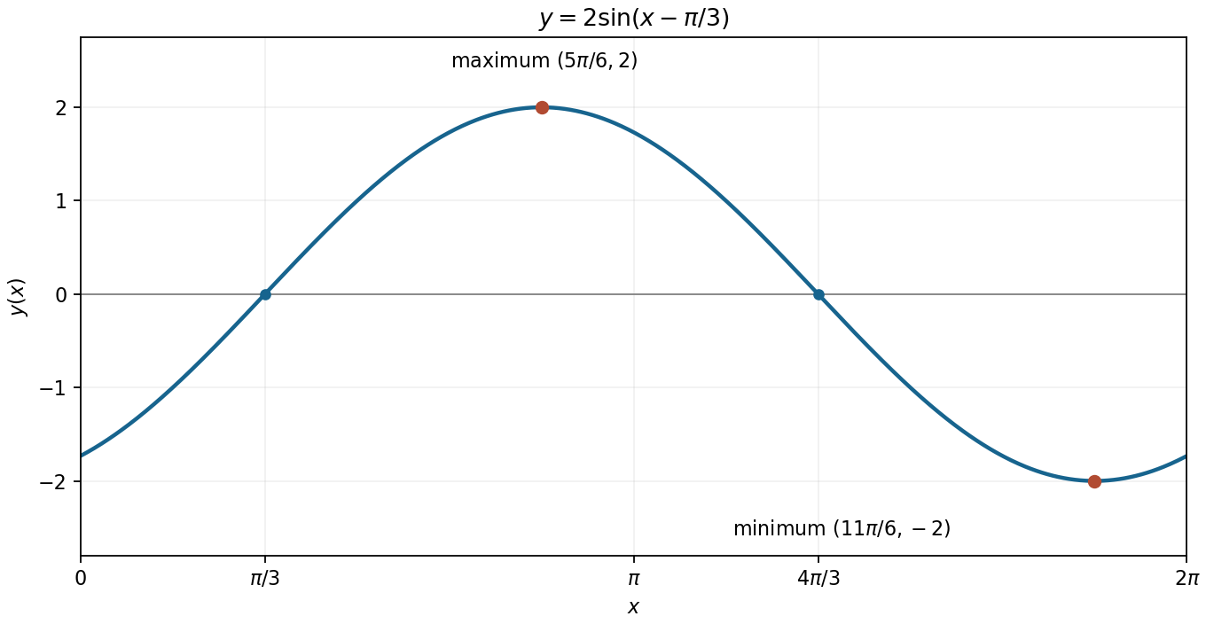
The unique periodic sinusoidal response, with its maximum, minimum and zero crossings
. Details. Past exam of the mathematics course of the year 1 of the natural sciences course of the University of Cambridge 2011 Paper 1 14 e Solution by Codex 0 2026-10-18
Codex 0 2026-10-18Using the sine addition formula, combine the surviving modes:It has amplitude and a phase delay . The full general solution would add , but this exponential is periodic only for , so the displayed periodic solution is unique.
Past exam of the mathematics course of the year 1 of the natural sciences course of the University of Cambridge 2011 Paper 1 14 d Solution by Codex 0 2026-10-18
Codex 0 2026-10-18The constant coefficient is . For every the two mode equations arewhere is the Kronecker delta. The first equation gives , so the second becomes . HenceNo other modes survive. This is the single-frequency case of the Fourier solution of a first-order equation with periodic forcing.
Past exam of the mathematics course of the year 1 of the natural sciences course of the University of Cambridge 2011 Paper 1 14 c Solution by Codex 0 2026-10-18
Codex 0 2026-10-18Fourier orthogonality isolates a coefficient. Multiplication by and integration over annihilates the constant, all cosine terms and all sine terms except the one with , whose squared integral is . Thus the corresponding coefficients on the two sides must agree for each positive integer .
Multiplication by works in the same way, while integration against the constant mode extracts . This is the uniqueness of the Fourier coefficients; it does not follow from comparing a few point values of the series.
Past exam of the mathematics course of the year 1 of the natural sciences course of the University of Cambridge 2011 Paper 1 14 b Solution by Codex 0 2026-10-18
Codex 0 2026-10-18Differentiate the Fourier series term by term and collect cosine and sine terms. Substitution into the equation givesFor a smooth periodic solution, differentiation of the series is justified. Alternatively, multiply the differential equation by each trigonometric mode and integrate by parts; periodicity cancels the boundary terms and gives the same coefficient constraints without first differentiating an infinite sum.
Past exam of the mathematics course of the year 1 of the natural sciences course of the University of Cambridge 2011 Paper 1 14 a Solution by Codex 0 2026-10-18
Codex 0 2026-10-18In the real Fourier series convention for period ,where the Fourier coefficients areThese formulas apply to integrable periodic functions. Writing equality at each point requires appropriate convergence hypotheses; the periodic solution sought below is smooth, so its series causes no such difficulty.
Pinned article: Introduction to the OurBigBook Project
Welcome to the OurBigBook Project! Our goal is to create the perfect publishing platform for STEM subjects, and get university-level students to write the best free STEM tutorials ever.
Everyone is welcome to create an account and play with the site: ourbigbook.com/go/register. We belive that students themselves can write amazing tutorials, but teachers are welcome too. You can write about anything you want, it doesn't have to be STEM or even educational. Silly test content is very welcome and you won't be penalized in any way. Just keep it legal!
Intro to OurBigBook
. Source. We have two killer features:
- topics: topics group articles by different users with the same title, e.g. here is the topic for the "Fundamental Theorem of Calculus" ourbigbook.com/go/topic/fundamental-theorem-of-calculusArticles of different users are sorted by upvote within each article page. This feature is a bit like:
- a Wikipedia where each user can have their own version of each article
- a Q&A website like Stack Overflow, where multiple people can give their views on a given topic, and the best ones are sorted by upvote. Except you don't need to wait for someone to ask first, and any topic goes, no matter how narrow or broad
This feature makes it possible for readers to find better explanations of any topic created by other writers. And it allows writers to create an explanation in a place that readers might actually find it.
Figure 1. Screenshot of the "Derivative" topic page. View it live at: ourbigbook.com/go/topic/derivativeVideo 2. OurBigBook Web topics demo. Source. - local editing: you can store all your personal knowledge base content locally in a plaintext markup format that can be edited locally and published either:This way you can be sure that even if OurBigBook.com were to go down one day (which we have no plans to do as it is quite cheap to host!), your content will still be perfectly readable as a static site.
- to OurBigBook.com to get awesome multi-user features like topics and likes
- as HTML files to a static website, which you can host yourself for free on many external providers like GitHub Pages, and remain in full control

Figure 2. You can publish local OurBigBook lightweight markup files to either OurBigBook.com or as a static website.
Figure 3. Visual Studio Code extension installation.
Figure 5. . You can also edit articles on the Web editor without installing anything locally. Video 3. Edit locally and publish demo. Source. This shows editing OurBigBook Markup and publishing it using the Visual Studio Code extension. 
- Infinitely deep tables of contents:



All our software is open source and hosted at: github.com/ourbigbook/ourbigbook
Further documentation can be found at: docs.ourbigbook.com
Feel free to reach our to us for any help or suggestions: docs.ourbigbook.com/#contact