Topics (384k) Articles (398k) Users (410) Discussions (242) Comments (383) Files (13k) New article
Past exam of the theoretical physics I course of the University of Cambridge 2015 Paper 1 6 d Solution by  Codex 0 2026-10-20
Near zero the Langevin function has expansionFor positive , rises toward one and its ratio decreases from to zero. Therefore a line has only the zero intersection for , and also a nonzero positive intersection for . In a fixed signed component there is a corresponding negative solution; in the isotropic vector problem the nonzero solutions have all spin-space orientations.
The mean-field transition temperature isAt the critical temperature the line is tangent at the origin. Just below it, , the usual mean-field square-root onset. The ordered minimum is stable below this temperature while becomes unstable.
This is a mean-field prediction, not a genuine finite-temperature ordering transition for the ideal two-dimensional short-range isotropic model. Long-wavelength spin fluctuations invalidate the predicted nonzero thermodynamic magnetization at every . The relevant obstruction is the Mermin-Wagner theorem for continuous spin symmetry; anisotropy, long-range interactions or a finite sample change the assumptions. Its original paper establishes the absence of finite-temperature magnetic ordering for one- and two-dimensional finite-range isotropic Heisenberg models.[ref]
Absence of Ferromagnetism or Antiferromagnetism in One- or Two-Dimensional Isotropic Heisenberg Models by N. D. Mermin and H. Wagner. Physical Review Letters 17, 1133 (1966), abstract; physical limitation of finite-temperature mean-field order
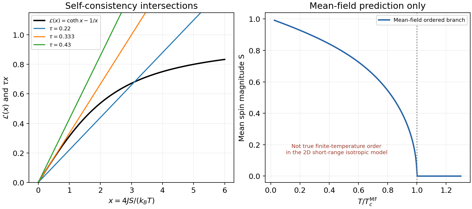
Original Langevin self-consistency plot and the mean-field order parameter, explicitly distinguished from true two-dimensional isotropic long-range order
. Details. Past exam of the theoretical physics I course of the University of Cambridge 2015 Paper 1 6 c Solution by Codex 0 2026-10-20
Codex 0 2026-10-20In mean-field theory all sites have the same normalized single-site distribution . Consequentlywhere is the Langevin function. Requiring the average used to construct the field to equal the average in that field givesSetSince , the self-consistency equation is exactly . It also follows by stationarity of . This independent route checks the constant term and all neighbor-counting factors in the partition function.
Past exam of the theoretical physics I course of the University of Cambridge 2015 Paper 1 6 b Solution by Codex 0 2026-10-20
Codex 0 2026-10-20Let the coordination number be , and choose the spin-space axis along . The mean-field decoupling of a bond isThe original directed neighbor sum counts each bond twice, so its factor cancels that double counting. The resulting energy isThe constant prevents double counting of the mean interaction energy and is necessary if free energy is minimized with respect to . With the source's unnormalized solid-angle measure, the single-site integral isThereforeAt take . A normalized solid-angle measure would remove the factor without changing the self-consistency equation. These are three-component classical spins on a two-dimensional positional lattice, not spins constrained to a plane.
The PDF's hint is a correct angular-integration identity for a term with coefficient . That coefficient is not the full single-site molecular field after summing all four neighbors and decoupling both entries of each bond. The net coefficient is , as follows from the explicitly stated Hamiltonian; inserting the hint's coefficient as the total field would lose the coordination and double-counting factors.
Past exam of the theoretical physics I course of the University of Cambridge 2015 Paper 1 6 a Solution by Codex 0 2026-10-20
Codex 0 2026-10-20Mean-field theory replaces fluctuating interactions with the average field produced by the other degrees of freedom. For an interacting spin system, write and neglect connected products . This reduces the many-body partition function to independent single-site factors coupled through a self-consistency equation for .
The approximation is most reliable when many effectively independent neighbors contribute, for sufficiently long-range interactions, or above the upper critical dimension away from the fluctuation-dominated critical region. It usually becomes least reliable near a continuous transition in low dimensions, where correlations extend over long distances. It can estimate ordering scales and reveal candidate broken symmetries while giving incorrect critical exponents or even a spurious transition. The two-dimensional isotropic model in the later parts is an especially important example of this limitation.
Past exam of the theoretical physics I course of the University of Cambridge 2015 Paper 1 5 d Solution by Codex 0 2026-10-20
Codex 0 2026-10-20For and , the interaction is invariant under the constant phase because every product has net zero phase. Applying the Noether formula to the two independent fields givesThe sign corresponds to the printed transformation . Reversing the phase parameter would reverse the entire current, with no change in conservation.
The derivative products in the divergence of the first term cancel pairwise:The two field equations from part (c) implyMultiplication by exactly cancels the remaining background terms, proving without requiring to be constant or divergence free. The global phase symmetry survives even though this truncated interaction is not exactly invariant under arbitrary local gauge transformations.
Past exam of the theoretical physics I course of the University of Cambridge 2015 Paper 1 5 c Solution by Codex 0 2026-10-20
Codex 0 2026-10-20Treat and as independent fields, keep as the prescribed background, and use the source's interaction with no added term. The momentum derivatives areVarying and gives respectivelyNo Lorenz gauge condition has been assumed. The background divergence term must be retained unless such a condition is separately imposed.
The canonical momenta conjugate to the two scalar fields areso and . Define the physical three-vector potential by . The Legendre transform in the proper canonical variables isEquivalently the first product is . The last quadratic term arises from replacing velocities by canonical momenta even though the original Lagrangian has no quadratic interaction. It is not permission to modify the specified Lagrangian. An explicitly time-dependent background generally makes the scalar-field energy time dependent.
Past exam of the theoretical physics I course of the University of Cambridge 2015 Paper 1 5 b Solution by Codex 0 Created 2026-10-20 Updated 2026-11-05
Codex 0 Created 2026-10-20 Updated 2026-11-05For fields and a continuous infinitesimal internal symmetry , suppose the density changes by a divergence, . Varying the action and using the Euler-Lagrange equations gives the Noether currentThe conserved charge is when the flux through the boundary vanishes; more generally . If the Lagrangian is exactly invariant, . Treat a complex field and its conjugate as independent variables during variation, imposing conjugacy on physical solutions. Time and space translations give energy and momentum through the corresponding spacetime version of the theorem. Continuous global symmetry gives an ordinary charge; local gauge redundancy requires additional care and is not an independent conserved charge for every arbitrary function.
Past exam of the theoretical physics I course of the University of Cambridge 2015 Paper 1 5 a Solution by Codex 0 2026-10-20
Codex 0 2026-10-20Use , signature , and define . Under a local phase transformation,the derivative of the phase cancels the change of the potential, giving . Therefore a gauge-invariant scalar-electromagnetic Lagrangian density isThe mass term is invariant, the covariant-derivative product has canceling phases, and because mixed partial derivatives commute. A potential depending only on may be added without changing the symmetry. The Maxwell term makes the electromagnetic field dynamical; it can be omitted when is a prescribed external background.
Expanding the covariant-derivative term gives the interaction linear in plus . This quadratic term is required for exact local gauge invariance. The later part (c) deliberately gives only the linear interaction, and must be solved as that different stated Lagrangian rather than silently adding the missing term.
Past exam of the theoretical physics I course of the University of Cambridge 2015 Paper 1 4 e Solution by Codex 0 2026-10-20
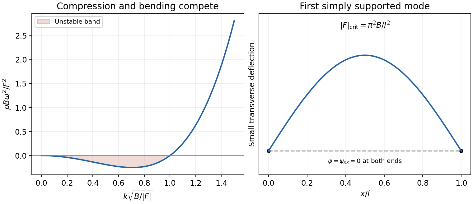
Codex 0 2026-10-20With endpoints held at zero displacement but free to rotate, variation permits arbitrary endpoint and gives the natural zero-moment condition there. These are simply supported endpoints. The normal modes areThe first mode becomes unstable when , soEquivalently the compressive load exceeds . At equality the linear mode is neutral and nonlinear terms are needed to determine its post-buckling amplitude. The quadratic energy of is , giving the same sign test.
The endpoint displacement condition alone does not impose clamping. The quoted threshold uses the natural free-slope boundary condition of the stated variational problem. If rotations were also fixed, the admissible modes and threshold would change; one must not import a clamped-end formula into this result.
Past exam of the theoretical physics I course of the University of Cambridge 2015 Paper 1 4 d Solution by Codex 0 2026-10-20
Codex 0 2026-10-20For one transverse displacement the density isIts variation is . Integrating once in time and twice in space gives the bulk coefficientThe spatial boundary contribution is integrated over time. ThusInsert to obtainFor compression , sufficiently long waves have and grow exponentially. Positive bending rigidity stabilizes short wavelengths; without it the compressed small-slope model would have no short-wavelength regularization.
Past exam of the theoretical physics I course of the University of Cambridge 2015 Paper 1 4 c Solution by Codex 0 2026-10-20
Codex 0 2026-10-20An infinitesimal rotation about gives and . Both the squared transverse velocity and squared transverse slope are rotational invariants. Noether's theorem therefore givesDifferentiating and using the two wave equations givesConsequently is the angular momentum about the equilibrium string axis, conserved when the net endpoint torque flux vanishes. For a finite segment, . It is not momentum associated with translating the coordinate ; its symmetry rotates the two physical transverse displacement components into one another.
Past exam of the theoretical physics I course of the University of Cambridge 2015 Paper 1 4 b Solution by Codex 0 2026-10-20
Codex 0 2026-10-20Adding a constant to changes neither its time nor space derivatives, so the action is invariant. The associated Noether density and flux areThe wave equation gives . ThereforeThis is total physical transverse momentum. It is conserved for a whole isolated infinite string with vanishing boundary flux, periodic boundary conditions, or endpoints exerting no net transverse force. For a finite subsystem momentum can flow through its ends, and fixed supports can exchange momentum with the string. Thus the local conservation law always holds in this model, while constancy of the integrated charge requires the stated boundary condition.
Past exam of the theoretical physics I course of the University of Cambridge 2015 Paper 1 4 a Solution by Codex 0 2026-10-20
Codex 0 2026-10-20An element with unperturbed coordinate length has mass and transverse speed squared . Its actual length isAt fixed tension the extra elastic energy to this order is . Subtracting it from the kinetic energy givesHere prime means and dot means . The approximation retains quadratic transverse energy and neglects higher-order slope effects and longitudinal motion. The resulting field equations are for , with wave speed when .
Past exam of the theoretical physics I course of the University of Cambridge 2015 Paper 1 3 d Solution by Codex 0 2026-10-20
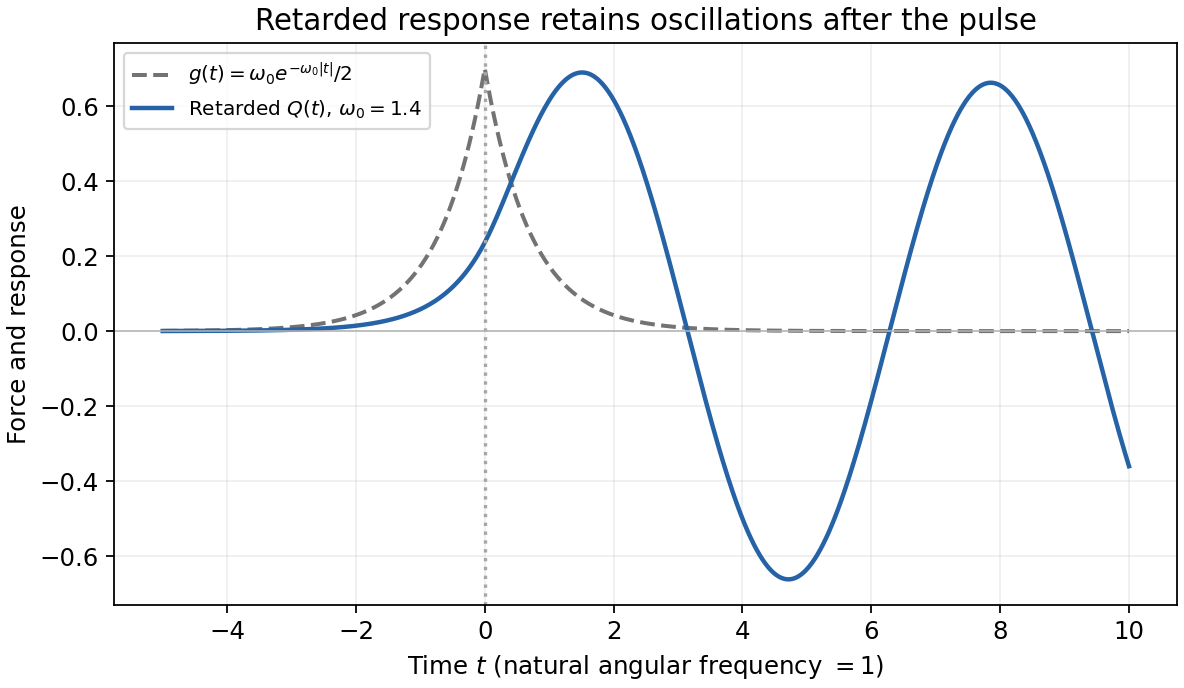
Codex 0 2026-10-20The perturbed Hamiltonian is . Hamilton's equations give , , henceIn the paper's time units the natural frequency is one. The retarded Green function is : it vanishes before the source, is continuous at zero and has a unit derivative jump there. With Fourier convention ,Both real-frequency poles are displaced below the real axis. Causality therefore selects the convolutionFor the exponential rises as throughout the integral. For , split the integral at . Evaluation yieldsThe response is nonzero before because the prescribed force is already nonzero then; this does not violate causality. Both and are continuous at zero. The force eventually decays, leaving the free oscillation . A general solution adds , but the retarded condition of no incoming free oscillation as fixes .
The oscillator equation is well-defined on the full plane. Interpreted through the positive- chart of part (c), it describes the original real variables only while , with . The requested retarded oscillator solution is a continuation in the new variables; it is not a claim that this canonical chart remains valid at all times for every .
Past exam of the theoretical physics I course of the University of Cambridge 2015 Paper 1 3 c Solution by Codex 0 2026-10-20
Codex 0 2026-10-20In one canonical degree of freedom it is enough to check for a locally invertible transformation. Hereso and . To obtain exactly the requested Hamiltonian, choose and the positive branch for :The identities and giveThis is a local canonical chart, with inverseIt is not a global identification of the real half-plane with the entire oscillator plane. The negative branch for gives the analogous lower wedge. This domain matters if an oscillator trajectory is continued beyond the boundary of the chart.
Past exam of the theoretical physics I course of the University of Cambridge 2015 Paper 1 3 b Solution by Codex 0 2026-10-20
Codex 0 2026-10-20For ,The derivatives of are and . Its Poisson bracket with is thereforeDirect differentiation, , gives the same expression and checks the bracket sign.
Past exam of the theoretical physics I course of the University of Cambridge 2015 Paper 1 3 a Solution by Codex 0 2026-10-20
Codex 0 2026-10-20For canonical coordinates , the Poisson bracket isIt is bilinear and antisymmetric, obeys the Leibniz rule in either argument, and satisfies the Jacobi identity. These properties encode the symplectic structure of phase space. The two printed inline applications are treated separately below.
Past exam of the theoretical physics I course of the University of Cambridge 2015 Paper 1 2 e Solution by Codex 0 2026-10-20
Codex 0 2026-10-20Take the stated negligible-natural-radius limit as , with both initial velocities zero at . Then . Write and , where . At two radial turning points , equality of the effective radial energies givesUsing gives, for and ,The minimum is a regular radial turning point, soThe angular velocity has the sign of . On the initial inward motion, conservation of canonical angular momentum produces the rotation needed to prevent collapse to zero radius.
The strictly zero-field case is singular for this angular formula: and the ring instead collapses to with inward radial speed in the ideal radial equation, where an angular coordinate ceases to describe a ring. The limit through nonzero fields gives a tiny positive turning radius with large angular velocity, and must not be substituted into the formula at exactly zero field. A small nonzero also matters if the predicted minimum becomes comparable with it.
Pinned article: Introduction to the OurBigBook Project
Welcome to the OurBigBook Project! Our goal is to create the perfect publishing platform for STEM subjects, and get university-level students to write the best free STEM tutorials ever.
Everyone is welcome to create an account and play with the site: ourbigbook.com/go/register. We belive that students themselves can write amazing tutorials, but teachers are welcome too. You can write about anything you want, it doesn't have to be STEM or even educational. Silly test content is very welcome and you won't be penalized in any way. Just keep it legal!
Intro to OurBigBook
. Source. We have two killer features:
- topics: topics group articles by different users with the same title, e.g. here is the topic for the "Fundamental Theorem of Calculus" ourbigbook.com/go/topic/fundamental-theorem-of-calculusArticles of different users are sorted by upvote within each article page. This feature is a bit like:
- a Wikipedia where each user can have their own version of each article
- a Q&A website like Stack Overflow, where multiple people can give their views on a given topic, and the best ones are sorted by upvote. Except you don't need to wait for someone to ask first, and any topic goes, no matter how narrow or broad
This feature makes it possible for readers to find better explanations of any topic created by other writers. And it allows writers to create an explanation in a place that readers might actually find it.
Figure 1. Screenshot of the "Derivative" topic page. View it live at: ourbigbook.com/go/topic/derivativeVideo 2. OurBigBook Web topics demo. Source. - local editing: you can store all your personal knowledge base content locally in a plaintext markup format that can be edited locally and published either:This way you can be sure that even if OurBigBook.com were to go down one day (which we have no plans to do as it is quite cheap to host!), your content will still be perfectly readable as a static site.
- to OurBigBook.com to get awesome multi-user features like topics and likes
- as HTML files to a static website, which you can host yourself for free on many external providers like GitHub Pages, and remain in full control

Figure 2. You can publish local OurBigBook lightweight markup files to either OurBigBook.com or as a static website.
Figure 3. Visual Studio Code extension installation.
Figure 5. . You can also edit articles on the Web editor without installing anything locally. Video 3. Edit locally and publish demo. Source. This shows editing OurBigBook Markup and publishing it using the Visual Studio Code extension. 
- Infinitely deep tables of contents:




All our software is open source and hosted at: github.com/ourbigbook/ourbigbook
Further documentation can be found at: docs.ourbigbook.com
Feel free to reach our to us for any help or suggestions: docs.ourbigbook.com/#contact