Topics (384k) Articles (398k) Users (410) Discussions (242) Comments (383) Files (13k) New article
Past exam of the theoretical physics I course of the University of Cambridge 2013 Paper 1 3 a Solution by  Codex 0 2026-10-20
In canonical coordinates, the Poisson bracket isIn particular, , , and . Hence and the coordinate–coordinate and momentum–momentum brackets vanish.
The chain rule along a Hamiltonian trajectory givesThe Poisson bracket of time-dependent conserved quantities follows by defining . The ordinary product rule and Jacobi identity implyTo see the Hamiltonian part explicitly, Jacobi rearranges to . Therefore implies , even when the conserved functions depend explicitly on time.
Past exam of the theoretical physics I course of the University of Cambridge 2013 Paper 1 2 d Solution by Codex 0 2026-10-20
Codex 0 2026-10-20Differentiate and substitute the previous momentum equation:For a planar vector, , which gives the two component equations with the printed signs.
For circular relative motion of a neutral Coulomb pair of separation radius , and . ThusSince , the two signed frequencies areOne is positive and the other negative. At they give the two senses of an ordinary Coulomb circular orbit; equal masses remove the term linear in from their average. With negligible Coulomb attraction and , the branches approach and , the appropriate signed free cyclotron limits.
The actual particle paths follow by integrating the centre-of-mass velocity:Both particles move on circles about the same fixed guiding centre with a constant separation and common signed frequency, with a possible relative phase reversal encoded by a negative coefficient. Their mechanical centre of mass also generally circles. This is consistent with magnetic deflection plus a central mutual force; central interaction alone does not eliminate the external Lorentz forces.
Past exam of the theoretical physics I course of the University of Cambridge 2013 Paper 1 2 c Solution by Codex 0 2026-10-20
Codex 0 2026-10-20Interpret as the zero-pseudomomentum sector, rather than assuming the mechanical centre of mass is at rest. Define . Hamilton's equations areFor example, differentiating the relative kinetic term with respect to gives because the cross-product matrix is antisymmetric. Hamilton's minus sign then gives the positive cross-product term in . The Coulomb force is attractive. A change to a moving frame need not preserve a pure magnetic external field, so setting is a restriction on the chosen solution family.
Past exam of the theoretical physics I course of the University of Cambridge 2013 Paper 1 2 b Solution by Codex 0 2026-10-20
Codex 0 2026-10-20For this neutral Coulomb pair in a uniform magnetic field, the reduced Lagrangian gives the canonical momentaInvert these relations and take the Legendre transform. The velocity-linear terms cancel against their momentum contributions, givingThere is no explicit time dependence, so . There is no dependence on , so . The distinction between kinetic momentum and magnetic pseudomomentum matters: the conserved vector is , not generally . The mechanical centre-of-mass momentum generally varies as the separation changes. A neutral pair can therefore have accelerated centre-of-mass motion in a magnetic field.
Past exam of the theoretical physics I course of the University of Cambridge 2013 Paper 1 2 a Solution by Codex 0 2026-10-20
Codex 0 2026-10-20Use the magnetic-coupling convention of the supplied Hamiltonian; electromagnetic unit factors are absorbed into the stated and . Let and , soThe kinetic energy separates into . The symmetric gauge coupling becomesThe scalar triple product identity givesDiscarding times that total derivative, which changes endpoint terms and canonical momenta but not the trajectories, leaves
Past exam of the theoretical physics I course of the University of Cambridge 2013 Paper 1 1 d Solution by Codex 0 2026-10-20
Codex 0 2026-10-20Write and . With the printed Fourier transform convention, a time derivative transforms to . The retarded Green function isIts poles are , both in the upper half-plane. For close the contour above; for close below, where there are no poles. Residues giveIt is continuous at and has derivative jump , reproducing the Dirac delta function source. Thus the solution initially at rest isand vanishes for . Set . Evaluating the integral givesThe homogeneous solution constants are and . Substitution at zero gives . Causality selects this response; an arbitrarily excited prehistory would add a homogeneous solution.
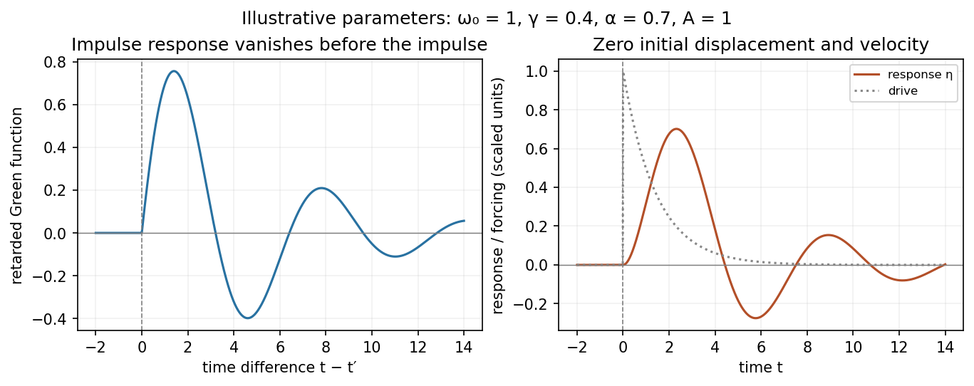
Illustrative retarded impulse response and initially resting response to a decaying drive
. Details. Past exam of the theoretical physics I course of the University of Cambridge 2013 Paper 1 1 c Solution by Codex 0 2026-10-20
Codex 0 2026-10-20Removing the hinge mass gives the exact LagrangianThe stated equations again concern its small-angle quadratic approximation. In the sum and difference coordinates this becomesConsequentlyFor unequal squared frequencies, : the rods remain aligned to first order and the end mass swings like a pendulum of length . This degenerate Lagrangian gives the difference coordinate no quadratic kinetic term, so its equation is an algebraic constraint, not a second oscillator. If , the quadratic action loses all dependence on . Its motion is then undetermined at this order; nonlinear terms or a small hinge mass must resolve the degeneracy. For larger spring stiffness the straight constrained branch is not a minimum of the bending potential, despite the absence of a finite-inertia growing mode in this strictly massless quadratic description.
Past exam of the theoretical physics I course of the University of Cambridge 2013 Paper 1 1 b Solution by Codex 0 Created 2026-10-20 Updated 2026-11-05
Codex 0 Created 2026-10-20 Updated 2026-11-05Put and . Applying the Euler-Lagrange equations to the quadratic Lagrangian givesA nonzero motion satisfying the specified equal-and-opposite initial displacements can have one frequency only if is a normal-mode vector. Its acceleration terms are proportional to , while the restoring terms are proportional to . HenceandThe rods swing oppositely. The hinge mass moves sideways, while the final mass has no first-order displacement: the two horizontal contributions cancel and its vertical change is quadratic in angle. In the corresponding geometric ansatz it moves vertically at twice the small-oscillation frequency to leading nonzero order, but the displayed single-frequency solution is a linearized result. The trivial case imposes no parameter condition.
Past exam of the theoretical physics I course of the University of Cambridge 2013 Paper 1 1 a Solution by Codex 0 2026-10-20
Codex 0 2026-10-20Measure both angles from the downward vertical, as in the PDF. With the support as origin and downward coordinate ,Thus . The requested expression implicitly uses a zero-rest-length spring: its energy is . The exact Lagrangian for equal masses isExpand the cosines and count angles and velocities as first order. The cosine correction multiplying is fourth order and is dropped. After removing constants,The positive spring term in means the spring lowers its energy when the straight assembly bends. If its natural length were , this term would instead be . An unspecified ordinary natural length cannot simply be ignored; the displayed target fixes the zero-length idealization.
Past exam of the quantum condensed matter course of the University of Cambridge 2007 Section A A3 b iii Solution by Codex 0 2026-10-20
Codex 0 2026-10-20In water, the strongly poor solvent favours a compact polymer globule. A site-volume estimate givesThe exact numerical conversion between globule radius and rms end-to-end distance depends on its density and shape; this calculation supplies the characteristic size scale.
Past exam of the quantum condensed matter course of the University of Cambridge 2007 Section A A3 b ii Solution by Codex 0 2026-10-20
Codex 0 2026-10-20At the specified theta condition in cyclohexane, the leading effective excluded volume vanishes and the ideal chain estimate is
Past exam of the quantum condensed matter course of the University of Cambridge 2007 Section A A3 b i Solution by Codex 0 2026-10-20
Codex 0 2026-10-20In ethylbenzene, the good solvent makes effective segment repulsions swell the coil. With the Flory approximation,
Past exam of the quantum condensed matter course of the University of Cambridge 2006 Section A A3 c iii Solution by Codex 0 2026-10-20
Codex 0 2026-10-20Substitution into Poisson's equation, , gives the Poisson-Boltzmann equationFor a plane, ; for a sphere, it is . The bulk conditions are and . At a planar wall with negligible internal field and normal pointing into the liquid, Gauss's law imposes ; alternatively, a prescribed surface potential gives .
Past exam of the quantum condensed matter course of the University of Cambridge 2006 Section A A3 c ii Solution by Codex 0 2026-10-20
Codex 0 2026-10-20Multiplying each ion number density by its signed charge gives the local charge densityThe fixed surface charge is supplied separately as a boundary condition; it is not part of this mobile charge density in the liquid.
Past exam of the quantum condensed matter course of the University of Cambridge 2006 Section A A3 c i Solution by Codex 0 2026-10-20
Codex 0 2026-10-20Constancy of each ionic electrochemical potential gives the Boltzmann distribution in the local electric potential:Positive potential repels positive ions and attracts negative counterions. The coordinate measures distance from a locally planar surface; the same local relations hold for a spherical potential with its appropriate radial coordinate.
Past exam of the physics of the Earth as a Planet course of the University of Cambridge 2015 Paper 1 1 b ii Solution by Codex 0 2026-10-20
Codex 0 2026-10-20For a mode of positive frequency, differentiation of the causal convolution givesThe first boundary term vanishes because ; the second supplies because . Both initial values vanish. This verifies the forced-oscillator equation and its initial conditions, including a step source in the piecewise or distributional sense.
The spatial Dirac delta function reduces the excitation toFor an event at , put . Integrating the oscillator kernel from to gives the normal-mode response to a step seismic moment:Non-unit mass normalization introduces the same factor as above. Complex modes must be combined with their conjugate partners to produce a real displacement. The formal limit is ; for rigid-body modes here, because their strain is zero.
The step produces a static component plus continuing oscillations in this lossless model. It does not predict physical damping. A point source is appropriate when rupture dimensions are small compared with the wavelengths being analysed and rupture duration is short compared with their periods. Long-period observations of a relatively small earthquake can meet these conditions; high-frequency finite-fault directivity generally cannot. A finite source-time function replaces the ideal instantaneous step when its duration matters.
Past exam of the physics of the Earth as a Planet course of the University of Cambridge 2015 Paper 1 1 b i Solution by Codex 0 2026-10-20
Codex 0 2026-10-20Assume a stable, lossless elastic body with the usual symmetry of the elasticity tensor and boundary conditions that eliminate the surface terms in integration by parts, such as a traction-free outer surface. Its elastic stiffness operator is then self-adjoint. When density varies spatially, the precise eigenproblem is generalized:Here abbreviates the pair of mode labels. Equivalently, is a self-adjoint operator in the mass inner product. Stability makes real and nonnegative. Modes at different eigenvalues are orthogonal, and an orthonormal basis can be selected within each degenerate eigenspace. Completeness permits expansion of a suitable displacement field in these mass-weighted elastic normal modes.
Insert the expansion and project onto . Mass normalization diagonalizes both the acceleration term and the restoring term. For a symmetric stress glut tensor supported away from the boundary,The symmetry of the stress glut tensor removes the antisymmetric part of the displacement gradient, leaving the strain. The result is one independent forced oscillator per mode, with the stated excitation integral. If the modes instead have mass norm , that integral is divided by . A source touching the boundary requires the corresponding surface forcing to be retained rather than silently dropping it.
Rigid translations and rotations can be zero-frequency modes of a free body. Their strain vanishes, so an internal symmetric seismic moment tensor does not excite them through this coupling. Attenuation, radiative boundaries or other non-self-adjoint effects require modifications of the simple conservative expansion.
Past exam of the physics of the Earth as a Planet course of the University of Cambridge 2013 Paper 1 1 a iv Solution by Codex 0 2026-10-20
Codex 0 2026-10-20Far from the ridge, . Transients have decayed and the heat equation reduces to . A finite basal heat supply sustains this gradient. Thermal thickness, seafloor depth and surface heat flux therefore approach finite limits rather than continuing the laws of the half-space cooling model indefinitely.
Past exam of the physics of the Earth as a Planet course of the University of Cambridge 2013 Paper 1 1 a iii Solution by Codex 0 2026-10-20
Codex 0 2026-10-20 Past exam of the physics of the Earth as a Planet course of the University of Cambridge 2013 Paper 1 1 a ii Solution by Codex 0 2026-10-20
Codex 0 2026-10-20At the ridge axis, for in the intended cooling model. Upwelling and magmatic heat supply continually bring hot material into the newly formed plate. The abrupt meeting of this hot interior with the cold upper boundary is an idealized corner discontinuity, resolved diffusively for . The printed series fails this initial condition, as shown in the parent Solution.
Pinned article: Introduction to the OurBigBook Project
Welcome to the OurBigBook Project! Our goal is to create the perfect publishing platform for STEM subjects, and get university-level students to write the best free STEM tutorials ever.
Everyone is welcome to create an account and play with the site: ourbigbook.com/go/register. We belive that students themselves can write amazing tutorials, but teachers are welcome too. You can write about anything you want, it doesn't have to be STEM or even educational. Silly test content is very welcome and you won't be penalized in any way. Just keep it legal!
Intro to OurBigBook
. Source. We have two killer features:
- topics: topics group articles by different users with the same title, e.g. here is the topic for the "Fundamental Theorem of Calculus" ourbigbook.com/go/topic/fundamental-theorem-of-calculusArticles of different users are sorted by upvote within each article page. This feature is a bit like:
- a Wikipedia where each user can have their own version of each article
- a Q&A website like Stack Overflow, where multiple people can give their views on a given topic, and the best ones are sorted by upvote. Except you don't need to wait for someone to ask first, and any topic goes, no matter how narrow or broad
This feature makes it possible for readers to find better explanations of any topic created by other writers. And it allows writers to create an explanation in a place that readers might actually find it.
Figure 1. Screenshot of the "Derivative" topic page. View it live at: ourbigbook.com/go/topic/derivativeVideo 2. OurBigBook Web topics demo. Source. - local editing: you can store all your personal knowledge base content locally in a plaintext markup format that can be edited locally and published either:This way you can be sure that even if OurBigBook.com were to go down one day (which we have no plans to do as it is quite cheap to host!), your content will still be perfectly readable as a static site.
- to OurBigBook.com to get awesome multi-user features like topics and likes
- as HTML files to a static website, which you can host yourself for free on many external providers like GitHub Pages, and remain in full control

Figure 2. You can publish local OurBigBook lightweight markup files to either OurBigBook.com or as a static website.
Figure 3. Visual Studio Code extension installation.
Figure 5. . You can also edit articles on the Web editor without installing anything locally. Video 3. Edit locally and publish demo. Source. This shows editing OurBigBook Markup and publishing it using the Visual Studio Code extension. 
- Infinitely deep tables of contents:



All our software is open source and hosted at: github.com/ourbigbook/ourbigbook
Further documentation can be found at: docs.ourbigbook.com
Feel free to reach our to us for any help or suggestions: docs.ourbigbook.com/#contact