Topics (384k) Articles (398k) Users (410) Discussions (242) Comments (383) Files (13k) New article
Past exam of the mathematics course of the year 1 of the natural sciences course of the University of Cambridge 2001 Paper 2 11 b i Solution by  Codex 0 2026-10-20
 Past exam of the mathematics course of the year 1 of the natural sciences course of the University of Cambridge 2001 Paper 1 12 c ii Solution by Codex 0 2026-10-20
Codex 0 2026-10-20For the standard normal density, . Using integration by parts,The boundary term vanishes because Gaussian decay dominates every power. Since the given mean is zero and variance is one, , yielding the Gaussian fourth moment
Past exam of the mathematics course of the year 1 of the natural sciences course of the University of Cambridge 2001 Paper 1 12 c i Solution by Codex 0 2026-10-20
Codex 0 2026-10-20The standard normal density is even, so is odd. Since Gaussian decay dominates every power, the integrand is absolutely integrable. Therefore
Past exam of the mathematics course of the year 1 of the natural sciences course of the University of Cambridge 2001 Paper 1 11 b ii Solution by Codex 0 2026-10-20
Codex 0 2026-10-20Write . Its cube roots have modulus two and arguments , for . ThusEach cube equals , and a cubic polynomial has no further distinct roots.
Past exam of the mathematics course of the year 1 of the natural sciences course of the University of Cambridge 2001 Paper 1 11 b i Solution by Codex 0 2026-10-20
Codex 0 2026-10-20In polar form, a cube root of one has modulus one and argument . The three roots of unity areThey are equally spaced on the unit circle.
Past exam of the mathematics course of the year 1 of the natural sciences course of the University of Cambridge 2001 Paper 1 11 a ii Solution by Codex 0 2026-10-20
Codex 0 2026-10-20The number has modulus one and argument modulo . Therefore its complex logarithm has valuesEvery value has real part zero. For the principal complex logarithm, choose the unique integer giving imaginary part in . The unwrapped value is the principal imaginary part only when it already lies in that interval.
Past exam of the mathematics course of the year 1 of the natural sciences course of the University of Cambridge 2001 Paper 1 11 a i Solution by Codex 0 2026-10-20
Codex 0 2026-10-20 Past exam of the mathematics course of the year 1 of the natural sciences course of the University of Cambridge 2001 Paper 1 10 a iii Solution by Codex 0 2026-10-20
Codex 0 2026-10-20The identity matrix has entries given by the Kronecker delta, soEach of the diagonal entries is one.
Past exam of the mathematics course of the year 1 of the natural sciences course of the University of Cambridge 2001 Paper 1 10 a ii Solution by Codex 0 2026-10-20
Codex 0 2026-10-20 Past exam of the mathematics course of the year 1 of the natural sciences course of the University of Cambridge 2001 Paper 1 10 a i Solution by Codex 0 2026-10-20
Codex 0 2026-10-20 Past exam of the mathematical and Computational Biology course of the University of Cambridge 2025 Paper 2 5 a ii Solution by Codex 0 2026-10-20
Codex 0 2026-10-20A day's admission count is a Poisson random variable with mean three. “Less than three” includes zero, one and two, soThus the probability is about .
Past exam of the mathematical and Computational Biology course of the University of Cambridge 2025 Paper 2 5 a i Solution by Codex 0 2026-10-20
Codex 0 2026-10-20The Waiting times of a Poisson process have an exponential distribution with the arrival rate. Measuring time in days, the survival function is . Thereforeor about .
Past exam of the mathematical and Computational Biology course of the University of Cambridge 2024 Paper 1 E8 e ii Solution by Codex 0 2026-10-20
Codex 0 2026-10-20For centred data, classical multidimensional scaling from Euclidean distances constructs the observation Gram matrixwhere . By part (i), its nonzero eigenvalues agree with those of , the matrix used for principal component analysis before dividing by a covariance normalization.
If is the unit observation-space eigenvector, the corresponding classical multidimensional scaling coordinate column isThat is exactly the column of principal component scores. Consequently classical multidimensional scaling of Euclidean pairwise distances recovers the same reduced coordinates as principal component analysis, up to signs and arbitrary orthogonal transformations within equal-eigenvalue subspaces. Distances alone cannot fix translation or orientation. The equivalence presumes centred data and Euclidean distances; general dissimilarities need not yield a positive semidefinite Gram matrix or a corresponding data covariance matrix.
Past exam of the mathematical and Computational Biology course of the University of Cambridge 2024 Paper 1 E8 e i Solution by Codex 0 2026-10-20
Codex 0 2026-10-20The premise contains a wording error: must be a nonzero eigenvalue, rather than a nonzero eigenvector. Let satisfyThen , since otherwise would force . Multiplying by givesThus , with eigenvector . Conversely, applying maps an eigenvector of with nonzero eigenvalue to one of .
These maps are inverses up to the factor on the corresponding eigenspaces, so the nonzero eigenvalues have equal multiplicities. Their zero eigenvalues need not have the same multiplicity because the two matrices can have different sizes. For a unit eigenvector and real , the normalized partner is , since .
Past exam of the mathematical and Computational Biology course of the University of Cambridge 2024 Paper 1 D6 b iii Solution by Codex 0 2026-10-20
Codex 0 2026-10-20For the Barabási-Albert model, choose a connected seed graph on vertices, the number of new edges per added vertex, and a final size . A complete seed with suffices. Add one vertex at a time, attaching it to distinct existing vertices selected with weights proportional to their current vertex degrees. Exclude duplicate edges and self-loops.
Increasing creates a larger network and permits older hubs to grow. Increasing makes the graph denser, with asymptotic average vertex degree , and tends to shorten graph distances. The seed affects early structure and the oldest hubs; standard linear preferential attachment gives a robust large-size tail exponent.
Its asymptotic degree distribution is , so it is a scale-free network. Hubs produce short average shortest path length, but elevated clustering coefficients are not automatic: with a tree seed gives a triangle-free tree, and clustering decreases with size in the standard model. The strict clustered small-world network property is therefore not guaranteed.[ref]
Emergence of scaling in random networks by Albert-László Barabási and Réka Albert. pp. 510–511, growth, attachment and degree exponent
Past exam of the mathematical and Computational Biology course of the University of Cambridge 2024 Paper 1 D6 b ii Solution by Codex 0 2026-10-20
Codex 0 2026-10-20For the Watts-Strogatz model, choose vertices on a ring, an even initial vertex degree , and a rewiring probability . Connect each vertex to its nearest neighbours on each side. Consider each original clockwise edge once: with probability , retain its starting endpoint and replace its other endpoint uniformly, excluding self-loops and duplicate edges. The edge count remains , although individual vertex degrees change.
Increasing at fixed lengthens unrewired-ring graph distances. Increasing adds edges and shortens distances. Increasing introduces shortcuts, sharply reducing average shortest path length at first, then progressively reducing the clustering coefficient by destroying local triangles.
The small-world network regime occurs at intermediate with sufficient shortcuts, substantial clustering, and . At distances are long; near the clustering advantage disappears. The degree distribution remains concentrated around , so this is not a scale-free network.[ref]
Collective dynamics of small-world networks by Duncan J. Watts and Steven H. Strogatz. pp. 440–441, construction and dependence on rewiring probability
Past exam of the mathematical and Computational Biology course of the University of Cambridge 2024 Paper 1 D6 b i Solution by Codex 0 2026-10-20
Codex 0 2026-10-20For the Erdős-Rényi model , choose the number of vertices and an edge probability . Visit every unordered pair of distinct vertices once and include its edge independently with probability . This construction gives a simple graph with expected edge count and mean vertex degree .
Increasing at fixed makes the graph denser, increases typical vertex degree and local clustering coefficient, and tends to shorten graph distances and improve connectivity. Increasing at fixed also increases the mean vertex degree; to retain a sparse comparison one instead decreases approximately as .
Its degree distribution is binomial distribution, approximately Poisson distribution in the sparse large- regime, so it is not a scale-free network. Connected realizations can have short average shortest path length, but their clustering coefficients are not elevated above the random baseline they themselves define. Thus they are not small-world networks under the high-clustering convention, although “small world” is sometimes used more loosely to mean only short distances.
Past exam of the mathematical and Computational Biology course of the University of Cambridge 2024 Paper 1 C5 c ii Solution by Codex 0 2026-10-20
Codex 0 2026-10-20For a haploid population with possible parents, each pair of ancestral lineages merges backward at rate in the Kingman's coalescent approximation. With lineages there are pairs. Hence the mean phylogenetic epoch duration isThus , and . For an autosomal sample from diploid individuals, replace the number of gene copies by , giving . A mitochondrial sample naturally uses a haploid maternal effective population size; the common factor cancels in the ratios below.
Past exam of the mathematical and Computational Biology course of the University of Cambridge 2024 Paper 1 C5 c i Solution by Codex 0 2026-10-20
Codex 0 2026-10-20In the Yule process, each of branches gives birth independently at rate per generation. The next birth therefore has total rate . Its waiting time has an exponential distribution, so the mean phylogenetic epoch duration isFor the ensuing calculation use , and . This is the inter-event waiting-time convention requested in the question, including an observation interval with four branches. Stopping the forward process immediately when the fourth branch is born would instead leave a zero terminal interval and describe a different sampling convention.
Past exam of the materials science course of the University of Cambridge 2022 Paper 1 6 c iii Solution by Codex 0 2026-10-20
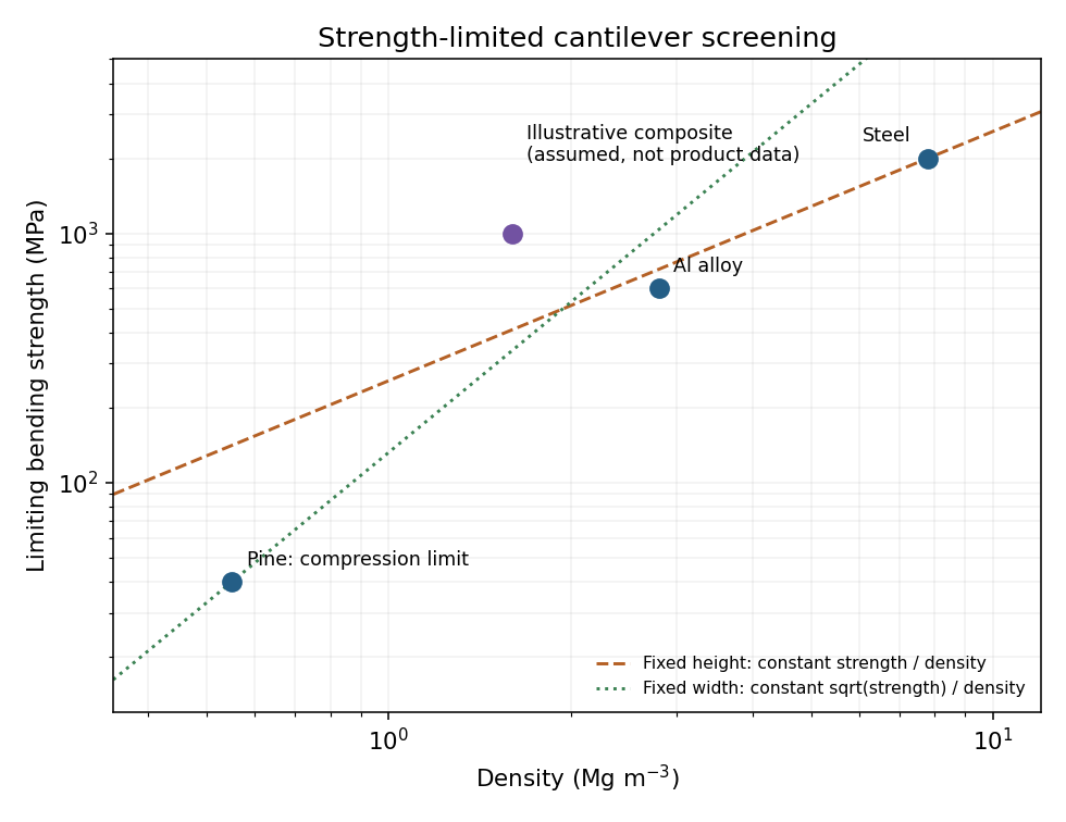
Codex 0 2026-10-20On a logarithmic strength–density materials selection chart, constant gives , a guideline of slope one; constant gives , of slope two. Moving each guideline upwards selects better candidates. A suitably qualified longitudinal carbon-fibre-reinforced polymer is a promising candidate for both designs. Composite families occupy favourable high-strength/low-density regions in published course selection charts, but a beam must meet its compressive as well as tensile allowable.[ref]
Examples of Materials Selection by Wright State University. Unit 5, strength–density charts and composite selection examples; family comparisons are screening evidence, not universal longitudinal compression data
Pinned article: Introduction to the OurBigBook Project
Welcome to the OurBigBook Project! Our goal is to create the perfect publishing platform for STEM subjects, and get university-level students to write the best free STEM tutorials ever.
Everyone is welcome to create an account and play with the site: ourbigbook.com/go/register. We belive that students themselves can write amazing tutorials, but teachers are welcome too. You can write about anything you want, it doesn't have to be STEM or even educational. Silly test content is very welcome and you won't be penalized in any way. Just keep it legal!
Intro to OurBigBook
. Source. We have two killer features:
- topics: topics group articles by different users with the same title, e.g. here is the topic for the "Fundamental Theorem of Calculus" ourbigbook.com/go/topic/fundamental-theorem-of-calculusArticles of different users are sorted by upvote within each article page. This feature is a bit like:
- a Wikipedia where each user can have their own version of each article
- a Q&A website like Stack Overflow, where multiple people can give their views on a given topic, and the best ones are sorted by upvote. Except you don't need to wait for someone to ask first, and any topic goes, no matter how narrow or broad
This feature makes it possible for readers to find better explanations of any topic created by other writers. And it allows writers to create an explanation in a place that readers might actually find it.
Figure 1. Screenshot of the "Derivative" topic page. View it live at: ourbigbook.com/go/topic/derivativeVideo 2. OurBigBook Web topics demo. Source. - local editing: you can store all your personal knowledge base content locally in a plaintext markup format that can be edited locally and published either:This way you can be sure that even if OurBigBook.com were to go down one day (which we have no plans to do as it is quite cheap to host!), your content will still be perfectly readable as a static site.
- to OurBigBook.com to get awesome multi-user features like topics and likes
- as HTML files to a static website, which you can host yourself for free on many external providers like GitHub Pages, and remain in full control

Figure 2. You can publish local OurBigBook lightweight markup files to either OurBigBook.com or as a static website.
Figure 3. Visual Studio Code extension installation.
Figure 5. . You can also edit articles on the Web editor without installing anything locally. Video 3. Edit locally and publish demo. Source. This shows editing OurBigBook Markup and publishing it using the Visual Studio Code extension. 
- Infinitely deep tables of contents:



All our software is open source and hosted at: github.com/ourbigbook/ourbigbook
Further documentation can be found at: docs.ourbigbook.com
Feel free to reach our to us for any help or suggestions: docs.ourbigbook.com/#contact