At the origin, the Poisson kernel is one, so the mean value property for harmonic functions givesFor $0<r<1$, the denominator in the Poisson kernel satisfies $1-2r\cos \vartheta +r^2\ge (1-r{)}^2$. ThusThe nonnegativity of $f$ allows this upper bound to be inserted under the Poisson integral on the unit disk:This is the upper bound in the Harnack inequality on the unit disk. The same argument with the minimum of the Poisson kernel gives the corresponding lower bound $(1-r)u(0)/(1+r)$.

Fix the observation point $\mathbf{x}$ and apply Green's second identity in the source variable $\mathbf{y}$. Since $\Delta u=0$, ${\Delta }_{\mathbf{y}}{G}_D={\delta }_{\mathbf{x}}$ and $G_D=0$ on the boundary, it givesThe identity can be justified by deleting a small circle about $\mathbf{x}$ and letting its radius tend to zero; the logarithmic flux contributes $u(\mathbf{x})$.

Set $\mathbf{x}=(r,\varphi )$ and $\mathbf{y}=(\rho ,{\varphi }^{\prime })$, and write $c=\cos (\varphi -{\varphi }^{\prime })$. The symmetric expression for the Green's function isAt the boundary, the outward normal derivative is ${\partial }_{\rho }$ at $\rho =1$, and henceSince $ds=d{\varphi }^{\prime }$ on the unit circle, the Poisson integral on the unit disk follows, with Poisson kernel

A Dirichlet Green function satisfies ${\Delta }_{\mathbf{x}}{G}_D(\mathbf{x},\mathbf{y})={\delta }^{(2)}(\mathbf{x}-\mathbf{y})$ in the domain and $G_D=0$ when $\mathbf{x}$ lies on its boundary. For a source $\mathbf{y}\ne 0$ in the unit disc, put its opposite image at ${\mathbf{y}}^{\ast }=\mathbf{y}/|\mathbf{y}{|}^2$. The method of images givesThe image lies outside the unit disc, so its logarithm is a harmonic function inside. The original logarithm has precisely the unit source strength found in part (a). On $|\mathbf{x}|=1$,so the boundary value is zero. Equivalently, in complex coordinates, the Dirichlet Green function inside the unit disk isThis also covers a source at the origin, where $G_D(z,0)=(2\pi {)}^{-1}\log |z|$.

Use the sign convention in which a fundamental solution of the Laplace equation satisfiesin the sense of distributions. It is a harmonic function away from the source. Writing $\rho =|\mathbf{r}-{\mathbf{r}}^{\prime }|$, the radial equation is $(\rho G^{\prime }{)}^{\prime }=0$, so $G=A\log \rho +B$. The divergence theorem on a small circle about the source fixes its total flux:ConsequentlyThe arbitrary constant is a harmonic function. For the alternative convention $-\Delta G={\delta }^{(2)}$, the logarithm has the opposite sign; subsequent Green's function formulas must use that convention consistently.

With $u=\cos \theta$, the boundary data have the finite Legendre polynomial expansionInside the sphere, every $r^{-\ell -1}$ term is singular at the origin and must be absent. Matching at $r=a$ therefore givesIn the exterior, decay at infinity excludes all $r^{\ell }$ terms, including the constant term at $\ell =0$. ThusBoth harmonic functions have the prescribed Dirichlet boundary condition, and each is finite throughout its own domain. The interior expression is regular even at the origin because $r\cos \theta =z$ and $r^2(3{\cos }^2\theta -1)=2z^2-x^2-y^2$. Uniqueness of the Dirichlet problem identifies these as the respective solutions. Their normal derivatives need not match: the two Dirichlet problems do not require a single harmonic function across the bounding sphere.

For a separated axisymmetric harmonic function $\Psi =R(r)\Theta (\theta )$, multiplying the Laplace equation by $r^2/(R\Theta )$ givesThe two sides depend on different variables, hence both equal a constant. Put $u=\cos \theta$ in the angular equation. Since $\sin \theta {\Theta }^{\prime }=-{\sin }^2\theta d\Theta /du$, it becomes the Legendre differential equationRegularity on both parts of the polar axis restricts $\lambda =\ell (\ell +1)$, with $\ell =0,1,\dots$, and selects the Legendre polynomial $P_{\ell }(u)$. The other angular solution is singular at an endpoint.

The radial Euler differential equation isTrying $R=r^s$ gives $s(s+1)=\ell (\ell +1)$, so $s=\ell$ or $s=-\ell -1$. Superposition of these separated harmonic functions givesThe Legendre polynomials form the angular expansion for regular data with rotational symmetry about the polar axis; the radial domain and the boundary conditions determine which coefficients survive and where the expansion converges.

For a finite group over $\mathbb{C}$, the number of inequivalent irreducible representations is its number of conjugacy classes, and the sum of squares of irreducible representation dimensions equals the group order. There are therefore five irreducibles for $S_4$, with squared dimensions summing to $24$.

First establish that part (c) found every one-dimensional representation. In such a representation, conjugate elements have the same scalar image. All transpositions are conjugate and square to the identity, so they all have one common image $s$ with $s^2=1$. Transpositions generate $S_4$, hence $s=1$ gives exactly the trivial representation, while $s=-1$ gives exactly the sign representation. There are precisely two degree-one irreducibles.

The other three dimensions $d_1,d_2,d_3$ are integers at least two and satisfyNo one of them can be at least four, since $4^2+2^2+2^2=24>22$. They are therefore all two or three. Starting from three twos gives sum of squares $12$; each replacement of a two by a three adds $5$. To reach $22$ requires exactly two replacements. Thus the complete list isThe count of conjugacy classes guarantees that these are all the inequivalent complex irreducible representations, not just dimensions of a proposed incomplete list.

The two one-dimensional representations are the trivial representation, ${\rho }_{+}(g)=1$, and the sign representation, ${\rho }_{-}(g)=\mathrm{sgn}(g)$. The first respects multiplication immediately. For the second, the sign of a permutation is the determinant of its permutation matrix, and multiplicativity of the determinant proves ${\rho }_{-}(gh)={\rho }_{-}(g){\rho }_{-}(h)$. They are inequivalent since a transposition has images $1$ and $-1$, and conjugation by a nonzero scalar cannot change a one-dimensional matrix.

Their group homomorphism kernels areBoth are subgroups, indeed normal subgroups, because they are kernels. In the second case $A_4$ is the alternating group of even permutations, with twelve elements.

The characters are their scalar values, since the trace of a one-dimensional matrix is its only entry. In the class order from part (b),The character inner product is the group average of ${\chi }_{+}\overline{{\chi }_{-}}$, soEach has squared norm $(1+6+3+8+6)/24=1$, in agreement with character orthogonality for distinct irreducible representations.

In a symmetric group, two permutations are in the same conjugacy class exactly when they have the same cycle type. For $S_4$ the five possibilities and their sizes areThere are $\left(\genfrac{}{}{0ex}{}{4}{2}\right)=6$ transpositions, three pairings into two unordered pairs, $\left(\genfrac{}{}{0ex}{}{4}{3}\right)(3-1)!=8$ three-cycles, and $(4-1)!=6$ four-cycles. Together with the identity these counts sum to $24=|S_4|$.

The symmetric group $S_n$ consists of all bijections of $\{1,\dots ,n\}$, with composition as its operation; its group order is $n!$.

An $m$-dimensional complex group representation of $G$ is a group homomorphism $\rho :G\to GL(V)$, where $V$ is an $m$-dimensional complex vector space. After a choice of basis, each $\rho (g)$ is an invertible $m\times m$ complex matrix, with $\rho (gh)=\rho (g)\rho (h)$.

An irreducible representation has $V\ne 0$ and no invariant vector subspace other than $\{0\}$ and $V$. Two group representations $\rho$ on $V$ and $\sigma$ on $W$ are isomorphic representations if there exists an invertible linear map $S:V\to W$ such that $S\rho (g)=\sigma (g)S$ for every $g$. They are inequivalent if no such map exists; in equal-dimensional matrix form this says no fixed change of basis conjugates every $\rho (g)$ to $\sigma (g)$.

The coefficient formula from part (b) and the Leibniz rule yield Rodrigues' formula directly:The leading coefficient is $(-1{)}^n/n!$, so $p_n^{(n)}=(-1{)}^n$. Substitute this differentiated expression into one factor in the squared weighted norm and apply integration by parts $n$ times:Every endpoint term contains a derivative of $e^{-x}{x}^n$ of order less than $n$: it vanishes at zero, and its exponential decay beats every polynomial at infinity. This proves the normalization of the ordinary Laguerre polynomials for all $n$, including $n=0$ without any integrations by parts.

The optimal approximation is the orthogonal projection onto the linear span of $p_0,\dots ,p_N$. Their orthogonality givesCompleting each square proves both optimality and uniqueness:For real $f$, these are real coefficients. If complex-valued $f$ is allowed while the coefficients remain real, replace the numerator by its real part and use the modulus-squared norm. The question's real formulation corresponds to real $f$.

Here the first three squared norms are one. Using ${\int }_0^{\infty }{x}^j{e}^{-2x}dx=j!/2^{j+1}$,Thus

Multiplication by a positive weight puts the differential equation into Sturm-Liouville form if $(xw{)}^{\prime }=(1-x)w$. Thus $x{w}^{\prime }=-xw$, and the constant factor can be chosen so thatThis fixes the otherwise arbitrary normalization of the weight consistently with the requested unit norms.

Write the polynomial as $p_n(x)={\sum }_{j=0}^n{c}_j{x}^j$. Comparing coefficients givesConsequently $c_j=(-1{)}^j(\genfrac{}{}{0ex}{}{n}{j})/j!$, identifying the solutions as Laguerre polynomials. In particular,Repeated integration by parts gives the moments ${\int }_0^{\infty }{e}^{-x}{x}^{j}dx=j!$. ThereforeFor later use, integration by parts in the weighted eigenvalue equations also givesThe endpoint expression vanishes because of the factor $x$ at zero and exponential decay at infinity. Hence distinct Laguerre polynomials are orthogonal, an instance of orthogonality of Sturm-Liouville eigenfunctions.

A weighted Sturm-Liouville operator has the formwhere $p,q,w$ are real, $p>0$ and $w>0$ in the interval's interior, and the coefficients have the regularity required by the derivatives. The corresponding eigenvalue equation is $-(p{y}^{\prime }{)}^{\prime }+qy=\lambda wy$. Its natural weighted inner product is $⟨f,g{⟩}_w=\int wf\bar{g}dx$. Suitable endpoint conditions must also annihilate $[p(f{\bar{g}}^{\prime }-f^{\prime }\bar{g})]$ for a self-adjoint differential operator; the displayed differential expression alone does not specify those conditions.

The original PDF places both endpoints at height $5/4$; the vertically stacked fraction can be misread in extracted text. The coefficient in the index is $4$, multiplying $\sqrt{y}$.

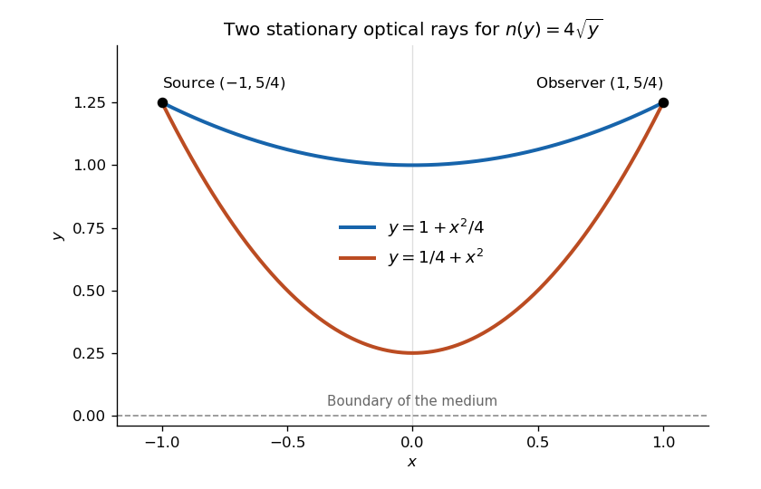
For the optical-length integrand $F=4\sqrt{y}\sqrt{1+y^{\prime 2}}$, the Beltrami identity applies because there is no explicit $x$ dependence. It giveswhere $h>0$ is constant. Therefore $y^{\prime 2}=y/h-1$. The full Euler-Lagrange equation is $2y{y}^{\prime \prime }=1+y^{\prime 2}$, and combining these gives $y^{\prime \prime }=1/(2h)$. This also excludes a constant curve, which would satisfy the squared first integral but not the full variational equation. Integration yieldsEqual endpoint heights at $x=-1,1$ require $x_0=0$. The height condition then becomes $h+1/(4h)=5/4$, or $4h^2-5h+1=0$. Its two positive roots are $h=1$ and $h=1/4$. Hence the two possible stationary rays areBoth stay in $y>0$, have the required endpoints and satisfy the variational equation. These are the two optical rays in a square-root refractive-index profile. Fermat stationarity supplies two rays; it does not assert that both globally minimize travel time.

Fermat principle states that the optical path length $\mathcal{S}=\int nds$, or equivalently travel time $\mathcal{S}/c_0$, is stationary under small variations of the ray with fixed endpoints. Stationarity need not mean a global minimum.

For a plane ray written as $y(x)$, use $\mathcal{S}[y]=\int F(x,y,y^{\prime })dx$, with $F=n(x,y)\sqrt{1+y^{\prime 2}}$. Its stationary paths obey the Euler-Lagrange equationIt follows by taking the first variation, integrating the term in $\delta y^{\prime }$ by parts, and using zero endpoint variations.

Use a Frobenius solution $y=x^{\sigma }{\sum }_{n\ge 0}{a}_n{x}^n$, with $a_0\ne 0$. The lowest power $x^{\sigma -1}$ has coefficient $2\sigma (2\sigma -1)a_0$, giving the indicial equationFor $n\ge 1$, matching the coefficient of $x^{n+\sigma -1}$ givesFor both candidate exponents the cancelled factor is nonzero in this range, so the recurrence isWith $a_0=1$, the exponent-zero solution isFor $\sigma =1/2$, the coefficients are $a_n=1/(2n+1)!!=2^{n}n!/(2n+1)!$, givingThe ratio test gives infinite radius of convergence for both series factors, since the successive ratios in magnitude are $|x|/(2n+2)$ and $|x|/(2n+3)$. The second full solution still needs a square-root branch in the complex plane; on $x>0$ it is a real solution. The distinct leading behaviors $1$ and $\sqrt{x}$ prove linear independence.

For an independent closed-form check on the structure, put $z=x/2$. The equation becomes $z{Y}^{\prime \prime }+(1/2-z)Y^{\prime }-(1/2)Y=0$, a Kummer differential equation with equal parameters. Its exponential reduction of a confluent hypergeometric equation with equal parameters explains the elementary first solution and the branched companion.

After normalization, $p=-6x^2/(1-x^3)$ and $q=-6x/(1-x^3)$. Both are analytic at zero, so $\boxed{x=0\text{ is ordinary}}$. At one,are analytic, whereas $p,q$ themselves have poles. Hence $\boxed{x=1\text{ is a regular singular point}}$.

Insert $y={\sum }_{n\ge 0}{a}_n{x}^n$. The coefficient of $x^0$ gives $a_2=0$; for $k\ge 1$ the coefficient of $x^k$ givesThus $a_n=a_{n-3}$ for $n\ge 3$. The initial data give $a_0=1$, $a_1=0$, soThe radius is one because the three cube roots of unity are poles of this solution. A direct structural check observes that the differential equation is exactly $[(1-x^3)y{]}^{\prime \prime }=0$. Thus $(1-x^3)y=A+Bx$, and the initial data select $A=1,B=0$. This is the product-derivative reduction of a second-order differential equation.