For an odd prime number $p$ and an integer $n$ not divisible by $p$, the Legendre symbol $\chi (n)=(n/p)$ is $1$ if $n$ is a quadratic residue modulo $p$, and $-1$ otherwise. One may extend it by $\chi (n)=0$ when $p\mid n$.

If a group representation of $G$ has character $\chi$, its restriction of a representation to $H$ has character $\chi {|}_H$. For an $H$-representation $V$ with character $\psi$, the induced representation is $\mathbb{C}[G]{\otimes }_{\mathbb{C}[H]}V$, with $G$ acting on the first factor. Decomposing into coset copies of $V$ shows that its character isIndeed only cosets fixed by $g$ contribute to the trace, and each coset has $|H|$ representatives.

The Frobenius reciprocity says $⟨{\mathrm{Ind}}_H^G\psi ,\chi {⟩}_G=⟨\psi ,{\mathrm{Res}}_H^G\chi {⟩}_H$. Directly, with the usual character inner product,The first equality substitutes $g=xh{x}^{-1}$ in the finite sum, and the second uses conjugacy invariance. This proves the theorem.

A matching in a graph from $X$ to $Y$ chooses one distinct neighbour in $Y$ for each vertex of $X$. For a finite bipartite graph, the Hall marriage theorem states that such a matching exists if and only if $|\Gamma (A)|\ge |A|$ for every $A\subseteq X$. Necessity follows because the matched neighbours of $A$ are distinct members of $\Gamma (A)$.

For sufficiency use induction on $|X|$, with the empty and one-vertex cases immediate. If some nonempty proper $A$ satisfies $|\Gamma (A)|=|A|$, the induced graph on $A,\Gamma (A)$ satisfies Hall's condition. The remaining graph on $X\setminus A,Y\setminus \Gamma (A)$ does too: for $B\subseteq X\setminus A$,Inductively match both pieces and combine them. If no nonempty proper subset is tight, choose an edge $xy$ and remove its endpoints. Every nonempty subset $B$ of the remaining $X$ is proper in the original $X$, so $|\Gamma (B)|\ge |B|+1$; removing $y$ preserves Hall's condition. Match the remainder inductively and add $xy$. This proves the theorem without a flow or disjoint-path theorem.

For a constant-density incompressible fluid, the Navier-Stokes equation and incompressibility constraint areScale length by $L_{\ast }$, velocity by $U_{\ast }$, time by $L_{\ast }/U_{\ast }$ and pressure by $\rho U_{\ast }^2$. In dimensionless variables they becomeA rectilinear flow has velocity $\mathbf{u}=U(y,z)\hat{x}$, parallel everywhere to one fixed direction and independent of that direction. Its convective acceleration is identically zero. A steady such flow therefore satisfies the linear equation $\nu {\Delta }_{\perp }U={\rho }^{-1}dp/dx$, with no inertial term and no Reynolds-dependent change of equation or spatial shape for fixed scaled boundary/forcing data. Relative changes in imposed pressure forcing can of course change the profile; Reynolds independence is not independence of the boundary data.

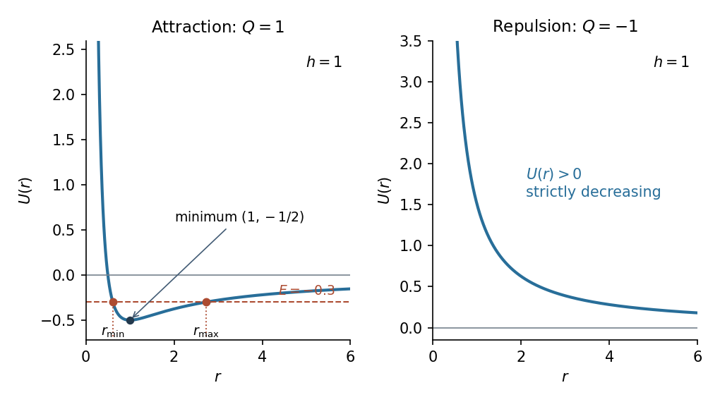
For the inverse-square potential $V(r)=-Q/r$, the central force is $-V^{\prime }(r)\hat{r}=-Q\hat{r}/r^2$. The transverse component of acceleration in polar coordinates is therefore zero:Thus $\boxed{h=r^2\dot{\theta }\text{ is constant}}$; for unit mass it is the signed angular momentum perpendicular to the orbital plane. The radial component givesConsequentlyThis is the mechanical energy, since the full kinetic energy is $\frac{1}{2}({\dot{r}}^2+r^2{\dot{\theta }}^2)$ and $r^2{\dot{\theta }}^2=h^2/r^2$.

For $h\ne 0$ and $Q>0$, the effective potential goes to $+\infty$ as $r\downarrow 0$ and to zero from below as $r\to \infty$. Its derivative is $U^{\prime }(r)=(Qr-h^2)/r^3$, so it decreases up to $r_0=h^2/Q$ and then increases. Its zero and minimum areFor $Q<0$, $U=h^2/(2r^2)+|Q|/r$ is positive and strictly decreasing, with limits $+\infty$ at zero and $0^{+}$ at infinity. It has no minimum at a finite positive radius.

If $h=0$, the centrifugal term disappears. For $Q>0$ the graph is instead $-Q/r$, increasing from $-\infty$ to $0^{-}$ without a minimum; for $Q<0$ it remains positive and decreasing. The bounded-orbit calculation below uses the stipulated $h>0$, which excludes this radial collision case.

Write ${\ell }_g$ for the dimensional offset of the centre of mass, reserving $h$ below for the dimensionless swimming parameter. The weight $-mg\mathbf{k}$ acts at $-{\ell }_g\mathbf{p}$, so its torque about the geometric centre is $mg{\ell }_g\mathbf{p}\times \mathbf{k}$. Buoyancy acts through the geometric centre and has no such torque. For a spherical cell, the ambient angular velocity is $\mathbf{\omega }/2$ and the rotational resistance is ${\zeta }_r=\rho \nu {\alpha }_{\perp }v$. Neglecting angular inertia, torque balance givesSince $\dot{\mathbf{p}}={\mathbf{\Omega }}_{\mathrm{cell}}\times \mathbf{p}$, the bottom-heavy spherical-cell orientation dynamics isThus a steady orientation satisfiesThe printed algebraic equation has the opposite sign on its right side, if vorticity means the usual $\nabla \times \mathbf{u}$. Its later concentration equation is consistent with the corrected sign. In particular, linearizing the corrected equation about $\mathbf{p}=\mathbf{k}$ gives ${\mathbf{p}}_{\perp }=(B/2)(\mathbf{\omega }\times \mathbf{k}{)}_{\perp }$, whereas the printed sign would reverse that response. Merely changing the definition of vorticity would also require changing the ensuing fluid and orientation calculations.

The gyrotactic reorientation time $B$ measures gravitational restoration against rotational viscous resistance. In still fluid a tilt angle obeys $\dot{\theta }=-\sin \theta /B$, soFor small tilt it is precisely the exponential relaxation time. Applying the algebraic orientation balance to a time-dependent disturbance additionally assumes that this relaxation is fast enough to neglect orientation lag. Keeping the full dynamic orientation equation would introduce an additional relaxation factor into the perturbation problem.

Suppress the common time factor $e^{i\omega t}$ and invert the stated Fourier transform with $(2\pi {)}^{-1}\int \Phi (k,y)e^{-ikx}dk$. Use limiting absorption principle $k_0\mapsto k_0-i0$, and choose $\gamma =\sqrt{k^2-k_0^2}$ with positive real part for the evanescent spectrum. For $|k|<k_0$ its outgoing continuation is $\gamma =+i\sqrt{k_0^2-k^2}$. The pole $-k_0$ lies above the inversion contour and $+k_0$ below it. These prescriptions fix both radiation and pole signs.

The even interior scattered transform solves ${\Phi }_{yy}-{\gamma }^2\Phi =0$, so it is $A(k)\cosh (\gamma y)$. The exterior transform is $B(k)e^{-\gamma (|y|-b)}$. Let $D^{-}(k)$ be the transform of their common upward normal derivative on $y=b$. On $x>0$ the rigid plates set both derivatives to zero; on $x<0$ continuity requires them to agree. Hence this derivative is supported on the negative half-line and is analytic below the transform contour. It follows thatThe difference between exterior and interior scattered traces on $y=b$ is $-D^{-}/L$, where $L=\gamma \sinh (\gamma b)e^{-\gamma b}$. At the open negative half-line the total traces must match, so this difference equals the incident wave $e^{i{k}_{0}x}$. Its negative-half transform is $-i/(k+k_0)$. The positive-half trace difference has an unknown upper-half-plane transform $C^{+}$, giving the Wiener-Hopf equationFactor $L=L^{+}{L}^{-}$, divide by $L^{-}$, and subtract the forcing pole using $C_0=L^{+}(-k_0)$:The left side is analytic below and the right side above; the pole in the last quotient is removable. Analytic continuation makes their common value entire. The finite-energy edge condition and algebraic factor growth make this entire remainder vanish: the allowed normal-velocity edge singularity is at most inverse-square-root, so its half-line transform is $O(|k{|}^{-1/2})$, while $L^{\pm }=O(|k{|}^{1/2})$. The same edge condition excludes a growing polynomial remainder. This pole subtraction in a Wiener-Hopf equation yieldsThe corresponding exterior result for the Wiener-Hopf solution for an open parallel-plate waveguide isBoth forms are useful: the first makes the common normal derivative transparent, and the second removes the apparent factor singularity at a grazing saddle.

The final unheaded request has a sign error in its printed exponent. To see this from the derived solution rather than an outgoing-decay assertion alone, simplify the interior transform toNear $k=-k_0$, $C_0/L^{+}(k)=1+O(k+k_0)$ and $e^{-\gamma b}\cosh (\gamma y)=1-b\gamma +O({\gamma }^2)$ for fixed $|y|<b$. ThusFor $x<0$, inversion of the first term gives $-e^{i{k}_{0}x}$, cancelling the continued incident potential. The remaining branch-point term uses $\gamma \sim i\sqrt{2k_0}(k+k_0{)}^{1/2}$ on the specified contour, so it is $b\sqrt{2k_0}(k+k_0{)}^{-1/2}$. Its inverse transform at $x=-r$ is proportional to $e^{-i{k}_{0}r+i\pi /4}/\sqrt{\pi r}$. Therefore the upstream decay of an open parallel-plate waveguide isThe amplitude decays as $(-x{)}^{-1/2}$, not $(-x{)}^{1/2}$. The positive exponent is present in the original PDF, so it cannot be proved under the stated outgoing problem. The incident pole cancellation and the explicit branch expansion give the corrected conclusion.

Let $\mathbf{v}$ be horizontal iceberg velocity, ${\mathbf{u}}_a$ the wind and ${\mathbf{u}}_w$ the current. Air and water drag forces act on the relative velocities, typically with magnitudes proportional to their squares. Their exposed and immersed areas and drag coefficients differ. For iceberg mass $m$, the horizontal balance can be written schematically aswhere $f$ is the Coriolis parameter and $\zeta$ the sea-surface elevation. The last term represents the large-scale pressure gradient; contact with pack ice and grounding require additional forces. Iceberg free drift neglects such contact constraints, not the water drag or Coriolis force.

In still water with a fixed wind force $\mathbf{F}$, a transparent transient model linearizes water drag as $-m\gamma \mathbf{v}$. Put $J\mathbf{v}=\hat{\mathbf{z}}\times \mathbf{v}$. ThenThe damped free drift of an iceberg isThus an initially resting berg accelerates under the wind, turns under the Coriolis force, and approaches a balance of wind, water drag and rotation through damped inertial oscillations. Its equilibrium drift is to the right of the wind in the Northern Hemisphere and to the left in the Southern Hemisphere. With quadratic drag, the drag coefficient in the equilibrium balance depends on speed; the linear formula illustrates the turning and relaxation rather than prescribing an exact percentage of wind speed.

For a moving ocean, the background pressure gradient associated with geostrophic balance must also be included. Large tabular icebergs have substantial submerged area and respond strongly to currents; smaller bergs can have a larger wind-driven velocity relative to the water. Near Antarctica, the mainly westward Antarctic Coastal Current can carry bergs along the continental margin. Export into offshore gyres and then the eastward Antarctic Circumpolar Current changes their trajectories; bathymetry, winds, fronts and evolving size all matter. Gladstone and Bigg's Weddell Sea tracking illustrates the contrast between coastal and offshore drift. The Antarctic Convergence separates colder Antarctic surface water from warmer water farther north, where an exported iceberg can encounter enhanced melting. No single wind direction determines the complete route.

The mechanisms affect surface energy input, heat supply from below, and the transport and thickness of sea ice. They reinforce one another: atmospheric warming and ocean heat thin the cover; circulation can export old ice; thinner ice melts earlier, increasing open-water absorption and strengthening ice-albedo feedback. Heat below the cold halocline matters only to the extent that mixing delivers it upward. Consequently the seven effects cannot be assigned independent percentages from the information given; their importance varies by region and year.

In a forward-looking answer from the paper's 2009 context, sustained warming would be expected to produce continued Arctic sea ice decline, a longer summer open-water season, less multi-year sea ice, and potentially nearly ice-free late summers within coming decades. Winter darkness permits new first-year sea ice to form, so loss of summer ice does not imply immediate year-round disappearance. Winter ice would tend to become thinner, more seasonal, and slower to recover after enhanced ocean heating. A precise date requires a forcing scenario and model, and internal variability causes year-to-year departures. Wang and Overland's 2009 projection is a contemporary example of such a conditional summer outlook.