Topics (384k) Articles (398k) Users (410) Discussions (242) Comments (383) Files (13k) New article
Past exam of the mathematics course of the University of Cambridge 2009 iii Paper 70 1 Solution by  Codex 0 2026-10-14
The axisymmetric magnetic mode spans a one-dimensional real representation of axial rotations, so its signed amplitude is a real variable . An equatorial dipole has two real horizontal components. Rotation through an angle rotates that pair; encoding the components by one complex amplitude gives , and rotation through gives . The velocity mode has the same rotational representation, so write it as . Magnetic reversal acts asThus the two relevant symmetries are axial rotation and magnetic reversal. Reflection symmetry has not been assumed, so complex coupling coefficients are permitted.
The equations for must be linear in the magnetic variables at fixed velocity. Combining this with rotational equivariance, their general local form iswhere is real valued and are complex valued. These functions can be understood through their local Taylor expansions; the symmetry argument does not require a convergent infinite series. Reality of explains its conjugate pairing.
For the velocity equation, a monomial must have the same rotational weight as and be even under magnetic reversal. Its selection rules areA formal sum of all such monomials with complex coefficients is the most general local velocity evolution. At degree one there is ; at degree two there is ; at degree three there are . Expanding the magnetic equations similarly gives the equivariant three-mode dynamo normal formThe are real, and the remaining coefficients are complex. The minus signs on cubic coefficients are a convention, not an assumption about their signs. Terms such as and are forbidden in the magnetic equations by magnetic linearity, even though symmetry alone would allow some of them.
For the normalization of nonzero dynamo coupling coefficients, assume . Make the variable changesThe transformed coefficients are and , of modulus one. ThusThe remaining phase is genuine; the two complex coefficients cannot both generally be made positive real. A zero coupling cannot be normalized to one, so the printed normalization presupposes this generic nonzero-coupling case.
Now impose the specified simplification, in the normalized variables, and write , with and signed real . Put . Separating real and imaginary parts givesConstant moduli require the first three right sides to vanish. Since , the first equation also fixes , so a continuously evolving phase difference must be constant. Hence the last right side must vanish as well. Both phases then advance at one common frequency, giving a relative equilibrium. These four algebraic conditions and the displayed common-frequency equations govern all the requested nonzero constant-modulus solutions, without needing to solve them.
The pure-velocity branch isThis presumes ; the usual saturated branch has . Near it, set , , and define and . Magnetic feedback in the velocity equation is quadratic, so the first magnetic linearization isA branch of the stated relative equilibria has a zero growth rate in this rotating frame. Its determinant therefore gives the magnetic onset on a rotating velocity branch conditionFor , the zero-mode relation is , so a nonzero gives a nonzero when . With a transverse eigenvalue crossing and nondegenerate nonlinear saturation this is the generic magnetic bifurcation surface; magnetic reversal pairs its two signs. Degenerate cases require separate treatment. For example, if and , determinant zero is automatic but the stationary equation forces , so that zero mode does not establish the requested branch with both magnetic amplitudes nonzero.
Past exam of the mathematics course of the University of Cambridge 2009 iii Paper 69 2 Solution by Codex 0 2026-10-14
Codex 0 2026-10-14Write the Bernstein basis as , with for out-of-range indices. The Bernstein polynomial isDifferentiation and the identities and give . Shifting the first sum's index therefore yieldsRepeating this calculation takes another forward finite difference of the coefficients and lowers the degree by one. Induction proves the derivatives of Bernstein polynomials formulaFor , define a continuous function on byAll sampled arguments lie in , since the largest is . At the degree- sampling point , this gives exactly the coefficient , and hence . The rescaling is essential: the sampling meshes are and , and the function depends on . For , the derivative is the constant , interpreted as a degree-zero Bernstein polynomial.
Now fix and assume . The supplied uniform limit of normalized finite differences, together with and uniform continuity of , shows thatPositivity and imply . For completeness, if then , and . Splitting according to whether and using Chebyshev's inequality givesFirst let and then ; this proves uniform convergence for each continuous . Finally,Thus Bernstein polynomial derivatives converge uniformly to the corresponding derivatives of , for each fixed with . Continuity of alone is sufficient for the definition of , but not for this derivative conclusion.
Past exam of the mathematics course of the University of Cambridge 2009 iii Paper 5 3 Solution by Codex 0 2026-10-14
Codex 0 2026-10-14Here is odd. For a finite p-group, write . A powerfully embedded subgroup satisfies ; this also makes normal, since every conjugate of an element of differs from it by an element of . A powerful p-group is one with , namely one powerfully embedded in itself. Use and throughout.
The lower p-series is defined byEach quotient is an elementary abelian p-group, and . These are generated subgroups, without closure bars, because the group is finite.
Past exam of the mathematics course of the University of Cambridge 2009 iii Paper 5 1 Solution by Codex 0 2026-10-14
Codex 0 2026-10-14A topological group is a group equipped with a topology for which multiplication and inversion are continuous maps. The product uses the product topology. Translation and inversion are therefore homeomorphisms. Hausdorffness is sometimes included in the definition; the two open-subgroup arguments below do not require it.
For the inverse system, take a directed set , topological spaces , and continuous maps for , with and . An inverse limit is a space with compatible continuous maps such that every compatible family factors uniquely as through a continuous map . Existence follows from the concrete constructionwith the subspace topology of the product topology. The only possible map is . Compatibility puts its image in , and coordinatewise continuity makes it continuous. This proves the universal property of an inverse limit, even when is empty. Given two inverse limits, their universal properties supply maps each way; the composites have the same coordinates as the identity, so uniqueness makes them identities. The inverse limit exists and is unique up to the unique homeomorphism respecting its projections.
A profinite group can be defined as an inverse limit of finite discrete groups, or as a compact Hausdorff space that is a totally disconnected space, equipped with continuous group operations. For the first implication, use the Tychonoff theorem. The compatibility equalities define a closed subgroup of the compact Hausdorff product. Two distinct points are distinguished by a finite discrete coordinate, so no connected subset contains both. Consequently the inverse limit is a compact Hausdorff totally disconnected topological group.
For the converse, use the topological result that a compact Hausdorff totally disconnected space has a basis of clopen sets. Choose a clopen set containing inside any specified identity neighbourhood. For each , continuity gives an identity neighbourhood and an open neighbourhood of with . Finitely many cover the compact set . Intersect their and its inverse to obtain a symmetric identity neighbourhood with . Symmetry also gives , and hence for every . The setis a subgroup containing , so it is open. It is contained in , since and . By part (ii), has finite index. Its normal core of a subgroup is a finite intersection of conjugates of , hence an open normal subgroup contained in . This proves the open normal subgroup basis of a profinite group.
The natural group homomorphismis injective because the intersection of these is . For a compatible family of cosets, any finitely many have nonempty intersection: their intersection subgroup is another indexing subgroup, and its prescribed coset lies in each. The finite intersection property and compactness give a point belonging to all the cosets, proving surjectivity. Finally a continuous bijection from a compact space to a Hausdorff space is a homeomorphism. The two definitions of profinite group are equivalent.
Past exam of the mathematics course of the University of Cambridge 2009 iii Paper 47 4 Solution by Codex 0 2026-10-14
Codex 0 2026-10-14An experimentally observed example of CP violation is the long-lived neutral kaon decay . The two-pion spin-zero final state is CP even, whereas would be the CP-odd neutral-kaon state in the CP-conserving limit. Its two-pion decay reveals CP violation. The historical experimental account is cern-courier.web.cern.ch/a/cp-violations-early-days/ .
For the CKM matrix, diagonalize the up- and down-quark mass matrices independently by biunitary transformations. Writewith and positive diagonal matrices. Only the left transformations enter the weak charged current, because its chiral projector removes the right-handed fields. Substitution givesThe matrix is unitary but need not be diagonal: the two left mass diagonalizations generally differ.
Using the field transformations in the subparts and reordering the anticommuting Dirac fields, the charged bilinear transforms aswhere the fields on the right are both evaluated at . The W boson contributes its second minus sign and Lorentz parity factor, so the product maps into its Hermitian-conjugate product. Crucially CP symmetry acts unitarily: it does not separately complex-conjugate the numerical coefficient . Thus the transformed interaction isComparing with the original interaction requires in this canonical CP convention. The physical condition is quark rephasing and CP conservation:A merely complex-looking matrix in an arbitrary mass-eigenstate phase convention is not itself proof of CP violation.
For CKM parameter counting, a unitary matrix has real parameters: mixing angles and phases. Rephasing the up and down mass eigenfields removes phases, since their common phase cancels out of . For generic nondegenerate masses this leavesThere is one physical phase for three families and none for one or two. Degenerate masses would permit additional transformations, so the generic count need not apply unchanged.
For the QCD part of the gauge covariant derivative, define the Hermitian colour matrix and chooseThis sign convention agrees with the field-strength definition in the source. The kinetic term contains . A vector bilinear under CP changes sign, gains the Lorentz parity matrix, and transposes its colour matrix upon exchanging quark and antiquark. Invariance of this interaction therefore requires the CP transformation of a non-Abelian gauge connection:Both the time/spatial distinction and the colour transpose are essential; individual colour components need not all share one charge-conjugation sign.
The same gauge covariant derivative givesApply the transformation above and the chain rule . The transpose reverses commutator order, , so the nonlinear term transforms with the same overall minus sign as the derivatives. This proves the CP transformation of non-Abelian field strength:Finally rewrites the theta density as . The two minus signs cancel, and transposition followed by cyclicity leaves the colour trace unchanged. But the four parity matrices acting on the Levi-Civita symbol contribute . HenceThe density is C even and P odd, therefore CP odd. A generic fixed nonzero theta coefficient violates CP symmetry. This is the source of the Strong CP problem, separate from the charged-current phase in the CKM matrix.
Past exam of the mathematics course of the University of Cambridge 2009 iii Paper 43 1 Solution by Codex 0 2026-10-14
Codex 0 2026-10-14A phase diagram partitions a space of control parameters into regions with distinct equilibrium phases. Its boundaries mark nonanalyticities of the thermodynamic-limit free energy; a first-order phase transition has a jump in a first derivative, whereas a continuous phase transition has a continuously vanishing order parameter and singular fluctuations.
An explicit three-parameter example is the scalar Landau free energywith parameter axes . These can be realized locally by the temperature, single-ion anisotropy and magnetic field of the Blume–Capel model. The three dimensions here refer to control-parameter space, not necessarily to three spatial dimensions. At , minimizing this potential gives a continuous phase transition at for . For , coexistence occurs at , whereThere are three global minima, and . Their order parameter jump decreases to zero as . Thus is a tricritical point. The two transition curves in the plane meet there.
In the three-dimensional phase diagram, crossing inside the ordered region switches between opposite signs of , so that region is itself a first-order phase transition sheet. For , two tricritical wings at opposite nonzero fields separate weakly and strongly magnetized phases. Their wing critical edges can be obtained rather than merely sketched: require . Since , the nonzero solutions satisfyThe fourth derivative there is , giving ordinary continuous critical endpoints. The wings meet the zero-field coexistence sheet along the tricritical three-phase line and terminate at these edges. Their exact tricritical wing coexistence factorization supplies the surfaces in the figure: for two nonnegative minima , set , andDirect expansion gives , proving that these surfaces describe coexistence of global, not merely local, minima.
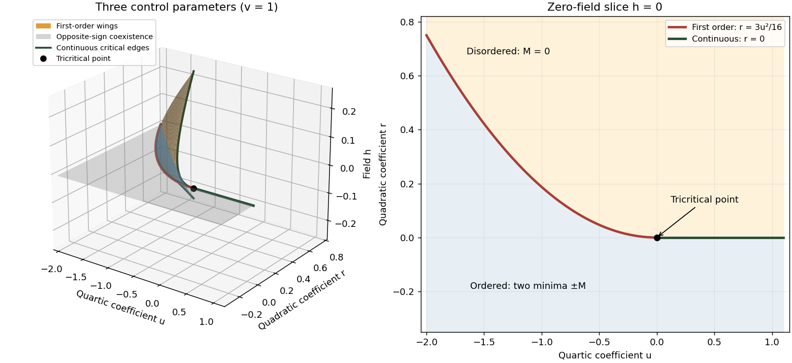
Tricritical phase diagram of the sextic scalar free energy: first-order sheets, critical edges and the zero-field slice
. Details. For the unheaded Ising model calculation, assume ferromagnetic exchange and let denote the mean Ising spin. On the hypercubic lattice the coordination number of a lattice is , even though the original positive-direction bond sum counts each bond only once. The mean-field approximation neglects products of deviations from :There are bonds, so the approximate energy is . Each independent Ising spin therefore sees the effective field . With , averaging its two Boltzmann weights gives the self-consistency equationThe slope of its right side at zero is , whereAbove , for excludes a nonzero solution. Below the initial slope exceeds one, and concavity of the hyperbolic tangent on the positive axis gives one positive solution and its negative partner. The Ising auxiliary mean-field free energy has positive quartic coefficient near , while its quadratic coefficient changes sign there. Its stable minima therefore move continuously away from zero; this is a continuous phase transition in the mean-field theory of the Ising model.
Put and . The Taylor expansion gives, on the nonzero branch,Consequently and the mean-field order-parameter exponent is . The inverse-temperature symbol used above is distinct from this order-parameter critical exponent.
Pinned article: Introduction to the OurBigBook Project
Welcome to the OurBigBook Project! Our goal is to create the perfect publishing platform for STEM subjects, and get university-level students to write the best free STEM tutorials ever.
Everyone is welcome to create an account and play with the site: ourbigbook.com/go/register. We belive that students themselves can write amazing tutorials, but teachers are welcome too. You can write about anything you want, it doesn't have to be STEM or even educational. Silly test content is very welcome and you won't be penalized in any way. Just keep it legal!
Intro to OurBigBook
. Source. We have two killer features:
- topics: topics group articles by different users with the same title, e.g. here is the topic for the "Fundamental Theorem of Calculus" ourbigbook.com/go/topic/fundamental-theorem-of-calculusArticles of different users are sorted by upvote within each article page. This feature is a bit like:
- a Wikipedia where each user can have their own version of each article
- a Q&A website like Stack Overflow, where multiple people can give their views on a given topic, and the best ones are sorted by upvote. Except you don't need to wait for someone to ask first, and any topic goes, no matter how narrow or broad
This feature makes it possible for readers to find better explanations of any topic created by other writers. And it allows writers to create an explanation in a place that readers might actually find it.
Figure 1. Screenshot of the "Derivative" topic page. View it live at: ourbigbook.com/go/topic/derivativeVideo 2. OurBigBook Web topics demo. Source. - local editing: you can store all your personal knowledge base content locally in a plaintext markup format that can be edited locally and published either:This way you can be sure that even if OurBigBook.com were to go down one day (which we have no plans to do as it is quite cheap to host!), your content will still be perfectly readable as a static site.
- to OurBigBook.com to get awesome multi-user features like topics and likes
- as HTML files to a static website, which you can host yourself for free on many external providers like GitHub Pages, and remain in full control

Figure 2. You can publish local OurBigBook lightweight markup files to either OurBigBook.com or as a static website.
Figure 3. Visual Studio Code extension installation.
Figure 5. . You can also edit articles on the Web editor without installing anything locally. Video 3. Edit locally and publish demo. Source. This shows editing OurBigBook Markup and publishing it using the Visual Studio Code extension. 
- Infinitely deep tables of contents:



All our software is open source and hosted at: github.com/ourbigbook/ourbigbook
Further documentation can be found at: docs.ourbigbook.com
Feel free to reach our to us for any help or suggestions: docs.ourbigbook.com/#contact