The partial correlation is the correlation of residuals after linearly projecting each of two variables on the conditioning variables and an intercept. With nonsingular covariance matrix, subtracting the two least-squares predictors gives residual covariance ${\sigma }_{12}-{\sigma }_{13}{\sigma }_{23}/{\sigma }_{33}$ and residual variances ${\sigma }_{ii}-{\sigma }_{i3}^2/{\sigma }_{33}$. Dividing gives the displayed formula. For a multivariate normal distribution, it is also the conditional correlation, independent of the conditioning value; this equality need not hold for general distributions.

The correlation coefficient computed under a conditional distribution, using its conditional covariance and positive conditional variances. It can depend on the observed conditioning value. For a multivariate normal distribution, conditioning on other coordinates gives the corresponding partial correlation.

The 2007 paper Comparison of the Hanbury Brown-Twiss effect for bosons and fermions by T. Jeltes and others compares polarized helium-3 fermions with helium-4 bosons. The chemical atoms occupy a metastable atomic level. Switching off magnetic trapping of neutral atoms releases them onto a microchannel plate detector with a delay-line anode, 63 cm below. Position and arrival-time readouts give three-dimensional pair separations by time-of-flight atom detection. About 1000 clouds per isotope supply histograms; normalization removes the broad cloud shape.

The pair detection correlation dips below one for helium-3 and rises above one for helium-4. The same apparatus, matched temperatures near $0.5\mu \mathrm{K}$, nearly identical trapping potentials, negligible interactions, and magnetic field gradient checks of spin polarization support an exchange-statistics interpretation. Finite detector resolution suppresses contrast; trap switch-off and resolution uncertainties limit quantitative agreement. A diverging laser lens deepens the dip, but its aberrations preclude a precise lens-model test. This detects exchange correlations, rather than measuring occupation of one selected spin orbital.^[ref]

For $M$ complete energy eigenstates of a one-particle Quantum Hamiltonian for identical noninteracting fermions, order their energies ${ϵ}_1\le \cdots \le {ϵ}_M$. At fixed particle number $0\le N\le M$, the Quantum Hamiltonian and the particle-number constraint areThe ground state occupies the $N$ lowest complete one-particle states. A short minimization argument suffices: moving an occupant from a higher energy to an empty lower energy decreases the total energy. This filling describes the ground state at temperature $T=0$; exclusion by itself also applies to excited quantum states and at positive temperature. The underlying thermal description is the Fermi-Dirac distribution.^[ref]

If the last occupied energy belongs to a group of $g$ one-particle states at the same energy and $q$ of them must be occupied, with all lower states filled, the ground state subspace has dimension $\left(\genfrac{}{}{0ex}{}{g}{q}\right)$. Exclusion does not select a particular basis or a particular quantum superposition in that subspace. The factor of two for an electron spatial orbital assumes both spin projections are included; a model restricted to one spin projection has only one state per spatial orbital. A magnetic field can split the degenerate energy levels, and interactions can change the lowest-energy electron configuration. Thus this finite noninteracting filling rule is not a complete prescription for interacting chemical atoms.

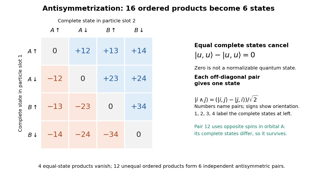
Exclusion constrains complete one-particle states, not a collection of little spatial boxes. In particular, two opposite-spin electrons in the same spatial orbital haveThe spatial factor is symmetric; the spin-one-half singlet state supplies the required antisymmetry. At ${\mathbf{r}}_1={\mathbf{r}}_2$, this wavefunction need not vanish for opposite spin labels. For equal spin labels it does vanish. In a continuous position description, an exact coincident point has zero measure anyway; the useful comparison concerns joint probability densities or detection in finite regions. Equal positions do not imply equal complete quantum states.

The fermionic occupation numbers $n_{\alpha }=0,1$ refer to a chosen orthonormal basis of one-particle states. A quantum superposition need not have definite occupation numbers in that basis, and an expectation value $⟨n_{\alpha }⟩$ can be fractional. For example, one electron in $(u+v)/\sqrt{2}$ has mean occupation number $1/2$ in each of two orthogonal spin orbitals, without splitting into two particles. The canonical anticommutation relations give $(a_{\alpha }^{†}{)}^2=0$ and make $a_{\alpha }^{†}{a}_{\alpha }$ a projector, so its expectation value stays between zero and one in every normalized quantum state.

The particle exchange operator $P_{12}$ swaps the complete particle slots, including spin. Its antisymmetric projector is $A_{12}=(I-P_{12})/2$. For orthonormal one-particle states $u,v$, the normalized multiparticle quantum state isBut attempting the same construction with $v=u$ gives the zero vector:The zero vector cannot be normalized to a quantum state. This is exclusion as cancellation of probability amplitudes, rather than a repulsive force. More generally, for normalized $u,v$ the squared norm of the numerator divided by $\sqrt{2}$ is $1-|⟨u|v⟩{|}^2$; the expression has unit norm only when $u,v$ are orthogonal. An overall quantum phase difference between $u,v$ describes the same one-particle state and also gives zero. Pauli explicitly connects exclusion with a vanishing antisymmetric wavefunction.^[ref]

A spatial orbital is a normalized spatial wavefunction used in a one-particle description. An atomic orbital is the corresponding notion for a chemical atom; a molecular orbital belongs to a molecule. A spatial orbital is not a trajectory and does not by itself specify spin.

A bit-flip channel applies the Pauli X gate with probability $p$ and does nothing otherwise. If the classical error outcome is not recorded, its output is the convex mixture ${\mathcal{E}}_p(\rho )=(1-p)\rho +pX\rho X$, not a coherent superposition of the two alternatives.

// Target: quantum-information-theory.bigb

Let $F/K$ be a finite Galois extension, choose a prime ideal $\mathfrak{q}$ above $\mathfrak{p}$, and write $k_{\mathfrak{q}}$ and $k_{\mathfrak{p}}$ for the residue fields. The decomposition group and inertia group areThe Frobenius automorphism on the finite field $k_{\mathfrak{q}}$ is $x\mapsto x^{N\mathfrak{p}}$. Its inverse image defines a distinguished coset in $D_{\mathfrak{q}}/I_{\mathfrak{q}}$; a Frobenius element is a lift of that coset. At an unramified prime, $I_{\mathfrak{q}}=1$ and the lift is unique. Changing the prime above $\mathfrak{p}$ conjugates it, so a Frobenius conjugacy class is intrinsically attached to $\mathfrak{p}$. These are arithmetic Frobenius conventions.

For a slender viscous thread, leading axial velocity is uniform over a section. Incompressibility gives $u_r=-r{w}_z/2$. The radial and azimuthal strain rates are $-w_z/2$, and the axial one is $w_z$. The Newtonian fluid stress tensor then has ${\sigma }_{rr}=-p-\mu w_z$. Matching the inviscid exterior normal stress requires $p=p_a-\mu w_z$, so ${\sigma }_{zz}=-p_a+3\mu w_z$. The coefficient three is the Trouton ratio.

A short section has end-stress resultant ${\partial }_z(A{\sigma }_{zz})dz$. The side's hydrostatic traction adds $p_a{A}_{z}dz$, and gravity adds $\rho gAdz$. Neglecting inertia and capillarity, their sum is zero:Since $(p_a{)}_z={\rho }_{a}g$, the balances areThe second is cross-sectional volume conservation, equivalently $D_{t}A=-A{w}_z$. Small interface slope justifies the sectionwise extensional approximation; the slow-flow assumption is additionally needed to neglect inertia.

The special unitary group is $\mathrm{SU}(2)=\{g\in M_2(\mathbb{C}):g^{\ast }g=I,\det g=1\}$. The special orthogonal group is $\mathrm{SO}(3)=\{R\in M_3(\mathbb{R}):R^{T}R=I,\det R=1\}$. Conjugation $A\mapsto gA{g}^{-1}$ preserves trace and skew-Hermiticity: for unitary $g$, $(gA{g}^{-1}{)}^{\ast }=g{A}^{\ast }{g}^{-1}=-gA{g}^{-1}$. It therefore defines the representation on the real space $V$ described in the following parts. The bar over the transpose in the PDF is essential; the condition is $A+A^{\ast }=0$, not ordinary antisymmetry over the complex numbers.

An orthonormal basis for the pairing proved below isPut $J_j=\sqrt{2}{E}_j$, so $J_j^2=-I$. For any unit real vector $v$, $J(v)={\sum }_j{v}_j{J}_j$ also squares to $-I$. Thus $g=\cos (\theta /2)I+\sin (\theta /2)J(v)$ belongs to $\mathrm{SU}(2)$. Conjugation fixes $J(v)$ and rotates its perpendicular plane by angle $\theta$ up to the orientation convention of this basis, as follows either by multiplying the displayed matrices or from their anticommutator relation $J(v)J(w)+J(w)J(v)=-2(v\cdot w)I$. Since every three-dimensional proper rotation has an axis and an angle, this proves surjectivity onto $\mathrm{SO}(3)$.

If an element is in the kernel, it commutes with each $E_j$. Commutation with $E_3$ forces it to be diagonal; commutation with $E_1$ forces its two diagonal entries to agree. Thus it is a scalar matrix, and determinant one and unitarity give exactly $\{I,-I\}$. Therefore $\boxed{\mathrm{SO}(3)\cong \mathrm{SU}(2)/\{\pm I\}}$.

The finite-dimensional complex irreducible representations of $\mathrm{SU}(2)$ are ${\mathrm{Sym}}^m({\mathbb{C}}^2)$, $m\ge 0$, of dimension $m+1$. The central element $-I$ acts by $(-1{)}^m$, so precisely the even ones descend. The irreducibles of $\mathrm{SO}(3)$ are $\boxed{{\mathrm{Sym}}^{2\ell }({\mathbb{C}}^2),\ell =0,1,2,\dots }$, viewed as representations of the quotient, with dimensions $2\ell +1$.

Fermat's little theorem states that for a prime $p$ and an integer $a$,Wilson theorem states that for a prime $p$,All the following modular congruences are taken modulo the indicated prime.

An inverse function of $f:X\to Y$ is a function $h:Y\to X$ satisfying bothThese are two-sided inverse identities. If $f(x)=f(x^{\prime })$, apply $h$ to get $x=x^{\prime }$, so $f$ is injective. For every $y\in Y$, the identity $f(h(y))=y$ supplies a preimage, so $f$ is surjective. Thus $f$ is a bijection.

Conversely, if $f$ is a bijection, each $y\in Y$ has exactly one preimage. Define $h(y)$ to be that preimage. Then $f(h(y))=y$ and $h(f(x))=x$, giving both identities. Hence a function has a two-sided inverse exactly when it is a bijection. This also makes its inverse function unique.

Let $dm$ be the gas mass ejected in a short interval, and let $dD$ be the stationary dust mass acquired. The rocket mass change is $dM=dD-dm$. Before the interval the momentum of the rocket and this dust is $Mv$, because the incoming dust is at rest. Afterwards it isto first order; changing the gas ejection speed by $dv$ affects only second-order terms. Momentum conservation, with no external force, therefore givesDividing by the time interval produces the rocket equation with stationary mass accretion:The incoming material's zero initial momentum is essential: accelerating it to the rocket's speed consumes part of the thrust.

Apply the rotating-frame derivative formula first to position and then to its inertial velocity:The angular velocity is constant, so there is no term involving $\dot{\mathbf{\omega }}$. By Newton's second law in the inertial frame, the inertial acceleration is $\mathbf{F}/m$. Rearrangement gives the equation of motion in a rotating frame:The two additional accelerations are the Coriolis acceleration and centrifugal acceleration.

For a nonzero complex number, write $z=r{e}^{i\theta }$ with $r=|z|>0$ and principal complex argument $-\pi <\theta \le \pi$. The principal complex logarithm and corresponding complex exponentiation areThe value at zero is not defined by this formula. The choice of complex argument matters: these are single-valued principal powers, rather than all values of a multivalued complex logarithm.

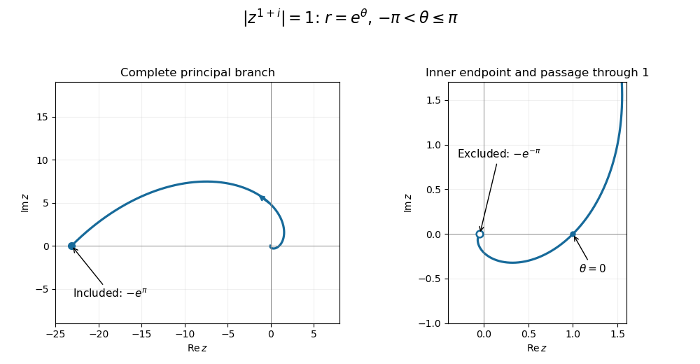
For the requested sketch, $(1+i)\mathrm{Log}z=(\log r-\theta )+i(\log r+\theta )$. Its complex exponential has complex modulus $e^{\log r-\theta }$, soThis is one turn of a logarithmic spiral, with increasing radius as the polar angle increases. It passes through $1$ at $\theta =0$, approaches the excluded endpoint $-e^{-\pi }$ from below the negative real axis, and ends at the included endpoint $-e^{\pi }$ from above that axis. The endpoint distinction follows from the chosen principal complex argument.

For the first additional construction, modify the rational/irrational example toAt zero, $|g(h)/h|=|h|\to 0$, so $g^{\prime }(0)=0$. At any nonzero point, density of the rational numbers and density of the irrational numbers give incompatible limiting values $x^2$ and $-x^2$. Thus $g$ is discontinuous, and hence not differentiable, there. Its differentiability set is exactly $\{0\}$.

For the second construction, use a summable absolute-value cusp series:On $[-R,R]$, each summand is bounded by $2^{-n}(R+1/2)$. The Weierstrass M-test therefore gives uniform convergence on every bounded interval, and the uniform limit theorem makes $G$ continuous everywhere.

To justify differentiability, each summand's difference quotient has absolute value at most $2^{-n}$, by the reverse triangle inequality. The sum of these bounds is finite, uniformly in the increment. Thus the tail of the difference quotient is uniformly small, and limits may be passed through the sum by first retaining finitely many terms and then making the tail small. If $x\ne 1/n$ for every $n\ge 2$, each individual summand is differentiable, givingIn particular $G^{\prime }(0)=-{\sum }_{n=2}^{\infty }{2}^{-n}=-1/2$. The accumulation of cusp locations at zero does not destroy the derivative, because their weights are summable.

At $x=1/m$, the same tail argument applies to both one-sided derivatives. Every term except the $m$th has the same derivative from both sides; the $m$th has derivatives $-2^{-m}$ and $2^{-m}$. ConsequentlyTherefore $G$ fails to be differentiable exactly at $1/2,1/3,1/4,\dots$, and is differentiable everywhere else.

The intermediate value theorem states that if $f:[a,b]\to \mathbb{R}$ is continuous, then every real value between $f(a)$ and $f(b)$ is attained at some $c\in [a,b]$. Here is a proof using completeness of the real numbers. Endpoint values are immediate, so suppose $f(a)<y<f(b)$; reversing the sign of $f$ handles the other ordering. LetThe set is nonempty and bounded above. Continuity at $a$ puts points to the right of $a$ in $S$, while continuity at $b$ excludes an entire interval to the left of $b$, so $a<c<b$. If $f(c)<y$, continuity puts some point larger than $c$ in $S$, contradicting its supremum. If $f(c)>y$, continuity excludes $S$ in a neighborhood of $c$, contradicting the existence of points of $S$ arbitrarily close to its supremum from below. Therefore $f(c)=y$, proving the theorem.

For the fixed-point assertion, put $g(x)=f(x)-x$. This is continuous, with $g(0)=f(0)\ge 0$ and $g(1)=f(1)-1\le 0$. If either endpoint value is zero it already gives a fixed point; otherwise the intermediate value theorem gives an interior zero. HenceThe proof needs both continuity and the closed-interval endpoint information; the following counterexamples separate those hypotheses.

Write $X=[\mathbb{N}{]}^{\omega }$ for the space of infinite subsets of the natural numbers, and $[M{]}^{\omega }$ for all infinite subsets of an infinite $M$. A family $Y\subseteq X$ is a Ramsey set of infinite subsets if for every infinite $M$ there is an infinite $L\subseteq M$ with either $[L{]}^{\omega }\subseteq Y$ or $[L{]}^{\omega }\cap Y=\varnothing$.

A non-Ramsey set of infinite subsets is obtained by finite-symmetric-difference parity colouring. Declare $A\sim B$ when their symmetric difference is finite, and use the axiom of choice to select a representative $R$ for each equivalence class. PutFor every infinite $L$, both $L$ and $L\setminus \{\min L\}$ belong to $[L{]}^{\omega }$ and have the same representative. Toggling one element changes the parity of the finite symmetric difference, so these two sets have opposite colors. Thus no $[L{]}^{\omega }$ is homogeneous, and $Y$ is not a Ramsey set of infinite subsets. Only finite differences are counted; no parity is being assigned to an infinite cardinal.

We use the Ellentuck topology for the star notation. Its basic neighborhoods arewhere $s$ is a finite stem (the initial segment of each member of the neighborhood) and every element of the infinite reservoir $A$ exceeds $\max s$; the empty stem is allowed. A star-nowhere dense set $N$ has star-closure with empty star-interior; a star-meagre set is a countable union of star-nowhere dense sets.

We need the following stem-preserving open-set conclusion: a star-open set $G$ has, in every $[s,A]$, an infinite $B\subseteq A$ such that $[s,B]\subseteq G$ or $[s,B]\cap G=\varnothing$. Here is the fusion proof for open Ellentuck sets, so that the precise form being used is explicit. A reservoir $T$ accepts a finite extension $t$ of $s$ when $[t,T]\subseteq G$, and rejects it when no infinite subreservoir accepts it. Every reservoir can be thinned to decide a prescribed stem: take an accepting subreservoir if one exists, and otherwise it already rejects. Acceptance and rejection are hereditary under further infinite thinning.

First thin $A$ to decide $s$. If it accepts, we have finished. Otherwise, choose successive points $b_0<b_1<\cdots$, thinning the unused tail after each selection to decide every stem $s\cup t$ with $t$ a subset of the finitely many points already selected. Each stage requires only finitely many decisions. The final set $B$ therefore decides every such finite extension, using the tail above its largest point. It rejects $s$.

For any rejected stem $s\cup t$, only finitely many possible next points $b$ of $B$ have accepting tails for $s\cup t\cup \{b\}$. Otherwise collect infinitely many such points into $C$. Every member of $[s\cup t,C]$ starts with some such $b$, and its remaining points lie in the accepting tail above $b$. Hence $[s\cup t,C]\subseteq G$, contradicting rejection. A second selection now gives $C\subseteq B$ all of whose finite extensions of $s$ are rejected: at each stage avoid the finitely many forbidden next points for each subset of the chosen prefix. Previous rejections persist on thinning. If $Z\in [s,C]\cap G$, star-openness gives an initial stem $s\cup t$ of $Z$ and an infinite tail of $Z$ whose entire neighborhood lies in $G$. This is an accepting subreservoir for a stem we made rejected, a contradiction. Thus $[s,C]\cap G=\varnothing$, proving the needed open-set conclusion.

Apply this conclusion to $G=X\setminus {\overline{N}}^{\ast }$ when $N$ is star-nowhere dense. This $G$ is star-open and star-dense. The alternative $[s,B]\cap G=\varnothing$ would give a nonempty star-open set inside ${\overline{N}}^{\ast }$, contradicting empty interior. Consequently every star-nowhere dense set can be avoided without extending the finite stem.

Now let $N={\bigcup }_{j\ge 0}{N}_j$, each $N_j$ star-nowhere dense, and fix $[s,A]$. Construct $b_0<b_1<\cdots$ with nested infinite unused reservoirs. At stage $j$, let $P_j=\{b_0,\dots ,b_{j-1}\}$. For every $t\subseteq P_j$, in turn, thin the current reservoir using the preceding avoidance property untilThere are only finitely many such $t$, and subsequent thinning preserves all previous avoidances. Choose $b_j=\min C_j$ and retain the part of $C_j$ above $b_j$ for the next stage. Put $B=\{b_j:j\ge 0\}$. For any $Z\in [s,B]$ and any $j$, the finite part $t=(Z\setminus s)\cap P_j$ is one of the stems tested at stage $j$, and the rest of $Z\setminus (s\cup t)$ lies in $C_j$. Hence $Z\in [s\cup t,C_j]$ and $Z\notin N_j$. This proves $[s,B]\cap N=\varnothing$.

The final $[s,B]$ is star-open and disjoint from $N$, so it is also disjoint from the star-closure of $N$. Every basic neighborhood therefore has a nonempty open refinement missing that closure. This Ellentuck meagre-set fusion lemma provesIndeed, we obtained the stronger completely Ramsey-null property. Testing all subsets of the selected prefix was essential; testing just the entire prefix would not cover every infinite subset of $B$.

Interpret the given relation by a subobject $R\hookrightarrow A\times B$ and write its projections as $p:R\to A$, $q:R\to B$. Totality says that the image of $p$ is all of $A$, so $p$ is a regular epimorphism. Single-valuedness makes $p$ monic: if $pr=ps$ for two arrows into $R$, the functionality sequent forces $qr=qs$, and the inclusion into $A\times B$ then gives $r=s$.

A regular epimorphism that is monic is invertible. Indeed its kernel pair consists of equal projections, and its coequalizer universal property supplies an inverse. Therefore defineThe graph of this map is exactly the original relation $R$, since $(p,q)=(1_A,f)p$. The graph also makes the map unique. This proves total functional relations define morphisms, using regular-category semantics and no choice of individual witnesses.