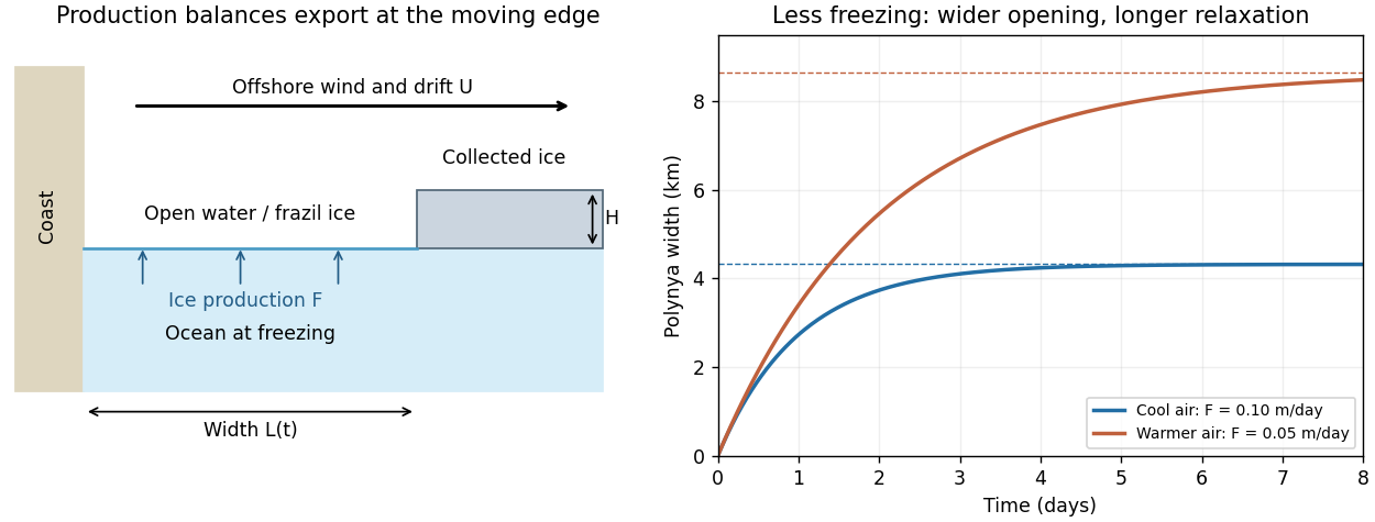
In the Pease polynya model, take a straight fixed coast at $x=0$ and an offshore polynya edge at $x=L(t)$. Let consolidated pack ice move offshore at speed $U>0$, let new ice be produced throughout the opening at equivalent thickness rate $F>0$, and let the collected ice at the edge have a prescribed thickness $H$. All fluxes below are per unit length of coastline. The new-ice volume production is $FL$, while the consolidated-ice export relative to the moving edge is $H(U-\dot{L})$. Neglect storage of drifting frazil ice inside the opening, so conservation givesThis is the simplest Pease closure: newly formed ice is collected at the edge rapidly enough that production can be equated to the instantaneous edge flux. A model retaining frazil storage would instead include the local balance ${\partial }_{t}h+{\partial }_x(uh)=F$, with frazil thickness $h$ and transport velocity $u$, together with an edge condition; it should not silently be identified with the instantaneous-collection approximation.

For constant $U,F,H$, the stable equilibrium and relaxation time areIn particular, an initially closed opening has $L(t)=L_{\infty }(1-e^{-t/\tau })$. It initially opens at speed $U$, then slows as its larger area produces more ice. It reaches $63\%$ of its ultimate width after $\tau$ and $95\%$ after $-\tau \log 0.05\simeq 3\tau$; the exact equilibrium is approached asymptotically, not reached at a finite opening time.

The production rate is determined by the energy budget. With $Q_{\mathrm{surf}}$ positive for net upward surface heat loss and $Q_o$ the heat supplied from the underlying ocean, water at its local freezing temperature givesThe surface loss includes sensible and latent turbulent transfers and net radiation. For example, the sensible component is approximately ${\rho }_a{c}_{p,a}{C}_{H}V(T_f-T_a)$, where $V$ is wind speed and $C_H$ an exchange coefficient. Ice motion is commonly parameterized as a small fraction of the offshore wind speed, but currents and the direction relative to the coast also matter. Thus colder air and stronger net cooling increase $F$ and narrow the opening; faster export increases $U$ and widens it; thicker collected ice increases both $L_{\infty }$ and $\tau$. Stronger winds can increase both export and heat loss, so the width's dependence on wind can be much weaker than the formula with artificially fixed $F$ would suggest.

The assumptions are steady spatially uniform forcing; a one-dimensional straight coast; fixed collection thickness and drift speed; no alongshore import of pack ice; water already at freezing rather than an appreciable sensible-heat reservoir; and negligible residence time of newly formed ice. Real coastlines, time-dependent winds, ocean currents, atmospheric adjustment over warm open water and variable ice accumulation can all violate these assumptions. The model describes a latent-heat polynya, not an opening maintained principally by a warm deep-ocean heat supply.

If air temperature rises while wind, $H$ and the other external parameters are unchanged, the smaller air–sea temperature difference reduces net heat loss and hence $F$. For $0<F^{\prime }<F$,The opening becomes wider and takes longer to attain the same fraction of its new equilibrium width. Its initial opening speed remains $U$; the longer equilibration follows from weaker ice production, rather than slower initial export. If warming eliminates net freezing, $F=0$ gives $L=L(0)+Ut$ in the simple kinematic closure, with no finite freezing-balanced width. A negative $F$ represents melt and is outside the positive-production Pease model.

For the shelf-water calculation, a $30$-day month at $0.05\mathrm{m}\mathrm{da}{\mathrm{y}}^{-1}$ produces $h_i=1.5\mathrm{m}$ of ice. Assume a well-mixed $D=100\mathrm{m}$ shelf column, no compensating advection or precipitation, and fixed ice and water densities ${\rho }_i=917$ and ${\rho }_w=1025\mathrm{kg}{\mathrm{m}}^{-3}$. The frozen fraction of its initial liquid mass isLet the liquid initially have salinity $S_0$, and newly formed ice retain $rS$ with $r=0.3$ and $S$ the instantaneous ambient value. For remaining liquid mass $M$, freezing removes salt with the departing ice, so conservation of salt with salt-retaining ice givesThereforeAn initial shelf-water salinity is needed for an absolute answer. Taking $S_0=34$ psu gives $\boxed{\Delta S\simeq 0.32\mathrm{psu}}$. At the accuracy of an equal-density thickness calculation, $f\simeq 1.5/100$ and $\Delta S\simeq 0.7S_{0}f$, giving about $\boxed{0.36\mathrm{psu}}$ for $S_0=34$ psu. These estimates describe the same modest increase. Treating ice as completely fresh would overestimate brine rejection by omitting the factor $0.7$.

The resulting water is denser and can leave the shelf and intrude beneath fresher surface water. It is therefore a physically plausible contribution to the cold halocline. Nevertheless, this one-month column budget yields only a few tenths of a psu, and the salinity contrast across the Arctic halocline can be several psu. If water from a shelf occupying one-third of the area were spread through an equally deep layer over the whole ocean, the average increase would be only about $0.1$ psu. This illustration is not a volume budget for the actual deep Arctic: shelf area fraction is not ocean water-volume fraction, and the exported water can be concentrated within a relatively thin halocline layer.

Consequently this calculation supports a shelf contribution but does not establish its dominance. Repeated seasonal ice production, enhanced production in polynyas, shelf-water export, freshwater dilution, and the thickness and residence time of the receiving layer would all be needed to test dominance. The assumption that the shelf initially becomes ice-free limits the first month's salt production; it does not bound an entire winter's cumulative production if new ice is continually removed.

Another pathway is winter cooling and limited convection of Atlantic-origin water as it enters the Arctic and encounters the ice-covered ocean. Cooling and local freezing can make it near-freezing water without requiring that it first be formed throughout the Siberian shelf. A subsequent fresh surface cap limits further convection; the cooled water is advected into the basin beneath that cap, producing a cold, salinity-stratified lower halocline. Pacific-origin waters also contribute to halocline structure in the western Arctic. Both formation and maintenance depend on circulation and freshwater supply, not simply on the presence of freezing somewhere. The strong stable density stratification then limits upward transfer of heat from the deeper Atlantic layer to sea ice.

Let the longitudinal variation scale be $\ell \gg h$. The stress-free boundary condition gives $\mu (u_z+w_x)=0$ at each face. Incompressibility implies $w=O(hu/\ell )$, so $w_x$ is smaller than a putative $u_z=O(u/h)$ by $O(h^2/{\ell }^2)$. The leading Stokes equation and the two shear-free conditions therefore make $u$ independent of $z$; its thickness-dependent correction is smaller-order. Symmetry gives $w=0$ at $z=0$, and incompressibility integrates toVertical momentum makes the leading normal stress independent of $z$. With the normal directed from liquid into gas, the upper-face curvature is $-h_{xx}/2$ to leading order. The Young–Laplace equation givesThe Newtonian fluid stress tensor also gives ${\sigma }_{zz}=-p+2\mu w_z=-p-2\mu u_x$. Hence $p=p_a-\gamma h_{xx}/2-2\mu u_x$ andThe factor four is the planar extension factor: both the longitudinal viscous stress and the pressure adjustment from transverse contraction contribute.

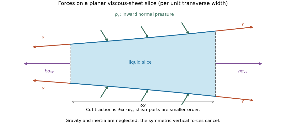
For force balance on the illustrated slice, the vertical cuts give $(h{\sigma }_{xx}{)}_x\delta x$. Pressure on the sloping broad faces gives $p_a{h}_x\delta x$ horizontally. Each of the two interfaces exerts a tangential surface tension pull at each cut, with horizontal component $\gamma \cos \theta$, where $\tan \theta =h_x/2$. Thus the horizontal force balance is the derivative of the effective tensionto the retained small-slope order. The ambient-pressure contributions cancel in this excess tension. Differentiating cancels the two $h_x{h}_{xx}$ terms, leaving the planar viscous-sheet stretching equationsThe upper-face kinematic condition is $w(x,h/2,t)=(h_t+u{h}_x)/2$. Combining it with $w=-z{u}_x$ gives the second equation,which is conservation of mass per unit transverse width.

For the two bubbles, let $p_g$ be the common gas pressure and $p_e$ the surrounding liquid pressure away from the sheet. A cylindrical bubble has one nonzero principal curvature, so the Young–Laplace equation gives $p_g-p_e\simeq \gamma /a$. In the nearly flat sheet the normal stress is $-p_g$, giving liquid pressure $p_{\mathrm{film}}=p_g-2\mu u_x$. The extensional correction is small compared with $\gamma /a$ because the transition scale will satisfy $\sqrt{a{h}_0}/L\ll 1$. Thus $p_{\mathrm{film}}\simeq p_g>p_e$, and this capillary pressure difference drives liquid out through both ends.

For a spatially uniform flat sheet, $h_x=h_{xxx}=0$, so the longitudinal equation gives $u_{xx}=0$. Reflection symmetry at $x=0$ selectsHere $U$ is the outward speed at the positive end. The mass equation then gives $h_t=-Uh/L$, independent of $x$, so initially uniform thickness remains uniform. Writing it as $h_0(t)$,The end transitions determine $U$, as derived in the following parts.

For an element $a$ of a complex unital Banach algebra, its spectrum of an element isThe nonzero spectra of products in opposite orders agree:For $\lambda \ne 0$, if $R=(\lambda 1-ab{)}^{-1}$ exists, direct multiplication on both sides verifiesInterchanging $a,b$ proves the converse. Zero may differ. On the Hilbert space ${\ell }^2({\mathbb{N}}_0)$, let $S$ be the unilateral shift operator $S{e}_n=e_{n+1}$ and take $a=S^{\ast }$, $b=S$. Then $ab=S^{\ast }S=I$, whereas $ba=S{S}^{\ast }=I-P_0$, where $P_0$ is projection onto the first coordinate. HenceBoth values for the second operator occur on its two nonzero invariant summands; every other value has an inverse obtained separately on those summands.

We use the spectral definition of a Positive element of a C-star algebra: $h$ is positive when $h=h^{\ast }$ and $\sigma (h)\subseteq [0,\infty )$. The continuous functional calculus, supplied by the Commutative Gelfand--Naimark theorem for the algebra generated by a Normal element of a C-star algebra and its adjoint, sends $F\in C(\sigma (h))$ to $F(h)$. It preserves products, sums, conjugation and the identity, is isometric, and satisfies $\sigma (F(h))=F(\sigma (h))$. For a self-adjoint element the spectrum is real, so real-valued functions produce self-adjoint elements.

For example, $F(t)=\sqrt{t}$ gives the positive square root in a C-star algebra of a Positive element of a C-star algebra. It satisfies $(h^{1/2}{)}^2=h$. Its uniqueness follows from the composition rule: if $d\ge 0$ and $d^2=h$, then the continuous functional calculus in the algebra generated by $d$ gives $\sqrt{d^2}=d$. For positive invertible $h$, the functions $t^{-1}$ and $t^{-1/2}$ give positive inverses and inverse square roots. If $0\le h$ and $r\ge \Vert h\Vert$, the function $r-t$ gives $r1-h\ge 0$; the same calculus givesThese transfer elementary scalar inequalities for functions of one element to the algebra. They do not justify applying a scalar inequality to arbitrary noncommuting elements.

To prove closure under addition without assuming an order theorem, let $a,b\ge 0$, set $\alpha =\Vert a\Vert$, $\beta =\Vert b\Vert$ and $s=\alpha +\beta$. If $s=0$, both elements are zero. Otherwise,The element $a+b$ is self-adjoint, so any $\lambda \in \sigma (a+b)$ is real and satisfies $|s-\lambda |\le s$. Thus $\lambda \ge 0$, provingWe will also use that the positive cone is proper: if $h\ge 0$ and $-h\ge 0$, then $\sigma (h)\subseteq \{0\}$, and the norm formula for self-adjoint elements gives $h=0$.

We next prove $a^{\ast }a\ge 0$ without presupposing that positivity is defined by such products. Put $h=a^{\ast }a$, which is self-adjoint, and form its negative part by the continuous functional calculus:This is positive. Let $c=a{h}_{-}^{1/2}$. Since $h_{-}$ commutes with $h$,The nonzero product-spectrum identity proved above gives $\sigma (c{c}^{\ast })\setminus \{0\}=\sigma (c^{\ast }c)\setminus \{0\}$. As $c{c}^{\ast }$ is self-adjoint, it too has spectrum in $(-\infty ,0]$, so $c{c}^{\ast }\le 0$.

Write $c=u+iv$ with $u=u^{\ast }$ and $v=v^{\ast }$. The continuous functional calculus makes $u^2$ and $v^2$ positive, and the addition result givesBut both summands on the left are nonpositive, so their sum is also nonpositive. Properness of the cone forces $c^{\ast }c+c{c}^{\ast }=0$. Now $c^{\ast }c=-c{c}^{\ast }$ is positive as well as nonpositive, so $c^{\ast }c=0$. The C-star identity gives $c=0$, whence $h_{-}^2=0$ and $h_{-}=0$. Thus $h$ has no negative spectral part:This proves the positivity of adjoint products from spectral positivity and the equivalence with the usual definition by elements of the form $d^{\ast }d$: the reverse direction is the factorization $h=(h^{1/2}{)}^{\ast }{h}^{1/2}$ for $h\ge 0$.

Finally, if $a\ge 0$ and $c\in A$, writeThe preceding result therefore provesIn particular, congruence preserves positivity in a C-star algebra, and $a\le b$ implies $c^{\ast }ac\le c^{\ast }bc$. These facts will justify the noncommutative order manipulations in the numbered parts.

A uniform algebra on a compact Hausdorff space $K$ is a closed complex subalgebra $A\subseteq C(K)$ containing the constants and separating points of $K$, with the supremum norm. It is therefore a commutative unital Banach algebra. Its character space of an algebra ${\Phi }_A$, also called its carrier space, consists of nonzero multiplicative linear functionals, equipped with the Gelfand topology.

For $x\in K$, evaluation gives the character of an algebra ${\delta }_x(f)=f(x)$. The map $\delta :K\to {\Phi }_A$ is continuous: composing it with the coordinate $\phi \mapsto \phi (f)$ gives the continuous function $f$ for every $f\in A$. It is injective because $A$ separates points. The Gelfand topology is Hausdorff because distinct algebra characters differ on some element of $A$. A continuous injection from compact $K$ into a Hausdorff space is a homeomorphism onto its image: closed subsets of $K$ have compact, hence closed, images. Its image is also compact and closed. Thusis the asserted homeomorphism. A natural uniform algebra is one for which this image is all of ${\Phi }_A$.

Use $\hslash =c=1$. For a canonical light scalar field with effective mass $m^2\ll H^2$, define the canonical Fourier mode $u_k=a\delta {\Phi }_k$. In the nearly de Sitter approximation it obeysDeep inside the Hubble radius, $k\gg aH$, the mode behaves like a Minkowski oscillator. Choosing the Bunch-Davies vacuum sets $u_k\to e^{-ik\eta }/\sqrt{2k}$. The normalized de Sitter solution isInflation stretches the physical wavelength until it exits the Hubble radius. For $|k\eta |\ll 1$, the growing scalar solution freezes with $|\delta {\Phi }_k{|}^2=|u_k/a{|}^2\to H^2/(2k^3)$. The dimensionless power spectrum is thereforeHere $H_k$ is evaluated when $k=aH$, since slow evolution near horizon exit fixes the frozen amplitude. Nearly constant $H$ and a light field make this spectrum almost scale-invariant; slow background evolution and small mass corrections produce a small tilt. The stretched vacuum modes supply the primordial stochastic fluctuations.

Expanding the covariant derivative isolates the ghost-gluon vertex interactionThe derivative acts on the antighost. With all momenta incoming, let its momentum be $k$, the gluon's Lorentz index be $\mu$, and their color indices be $(a,b,c)$ in the order $(\bar{c},A,c)$. The convention $e^{-ikx}$ replaces ${\partial }^{\mu }$ by $-i{k}^{\mu }$, and multiplication by $i$ from $e^{iS}$ givesMomentum conservation is implicit. The structure constants reflect the Adjoint representation, and the antighost momentum follows directly from its differentiated field. Reversing the momentum convention changes the displayed vertex sign consistently; exchanging the ghost and antighost source order also carries a fermionic sign.

The scaling hypothesis for critical phenomena says that the singular equilibrium free-energy density is a generalized homogeneous function of the thermal and field variables, after analytic backgrounds are removed. To derive the ordinary mean-field form, put $r=r_{t}t$, $u>0$ and neglect the higher powers near the transition. Rescale $m=\sqrt{r_t/u}|t{|}^{1/2}\psi$. Minimizing the quartic potential becomesThis is the mean-field scalar free-energy scaling form with $a=r_t^2/u$, $b=\sqrt{u}/r_t^{3/2}$. The two functions correspond to $t>0$ and $t<0$; the latter has two pure-phase branches and a cusp at zero field. The question's $>$ and $<$ subscripts distinguish these temperatures above and below $T_c$.

Differentiating with respect to $h$ gives $m=-{\partial }_h{A}_s\propto |t{|}^{1/2}$ on an ordered pure branch, and differentiating again gives $\chi =-{\partial }_h^2{A}_s\propto |t{|}^{-1}$. Thus the displayed scaling form independently yields $\beta =1/2$ and $\gamma =1$.

To allow anomalous powers, replace it byThen $\beta =2-\alpha -\Delta$ and $\gamma =2\Delta -(2-\alpha )$. Taking $t\to 0$ at fixed small $h$ gives $A_s\propto |h{|}^{(2-\alpha )/\Delta }$, so $1/\delta =(2-\alpha -\Delta )/\Delta =\beta /\Delta$. Eliminating $\Delta$ proves the Rushbrooke scaling relation and Widom scaling relation:These power-law relations assume the simple scaling form; marginal corrections or dangerously irrelevant couplings can require additional scaling variables.

The PDF gives an inverse-gamma distribution with shape $k$ and scale $\theta$, and a gamma distribution prior with shape $\alpha$ and rate $\lambda$. Write $\mu (\theta )=\theta /(k-1)$. The supplied conditional moments, together with $\mathbb{E}\theta =\alpha /\lambda$ and $\mathbb{E}{\theta }^2=\alpha (\alpha +1)/{\lambda }^2$, give the three structural quantities of the Bühlmann model:Here $v$ is the variance of hypothetical means and $s^2$ the expected process variance. The law of total covariance and conditional independence of different years implyAll these quantities are finite because $k>2$.

For any coefficients $c_i$, minimizing the mean squared error over the intercept first gives $c_0=m(1-{\sum }_i{c}_i)$. Let $Y=\mu (\theta )-m$ and $W_i=X_i-m$. Expanding the remaining mean squared error givesIts normal equations are $s^2{c}_i+v{\sum }_j{c}_j=v$ for every $i$. Since $s^2>0$, subtracting any two equations shows that all $c_i$ agree. The quadratic part is strictly positive for every nonzero coefficient change, so the solution is the unique global minimizer. Solving givesA credibility estimate combines individual experience with the collective expected value, using an experience weight $Z\in [0,1]$. In this equal-exposure setting, the Bühlmann credibility premium isThus the computed coefficients give exactly a credibility estimate, with a fixed credibility factor determined by known parameters and the number of observed years. This is Bühlmann credibility for inverse-gamma observations.

For the final Bayesian calculation, the likelihood function in $\theta$ is proportional to ${\theta }^{nk}\exp (-\theta {\sum }_i{x}_i^{-1})$. Multiplication by the gamma distribution prior gives the Gamma prior for an inverse-gamma scale updateUnder quadratic loss, the conditional risk of an estimate $d$ is $\mathrm{Var}(\mu (\theta )\mid x)+(d-\mathbb{E}[\mu (\theta )\mid x]{)}^2$. Its minimizer is therefore the posterior mean:This is not a fixed-weight arithmetic-mean credibility estimate. For $n=2$, the observations $(1,3)$ and $(2,2)$ have the same sample mean, but reciprocal sums $4/3$ and $1$, hence different posterior means. For any $n>2$, append the same positive observations to these two samples. For $n=1$, the estimate is $Cx/(1+\lambda x)$, with $C=(\alpha +k)/(k-1)$; its second derivative is $-2C\lambda /(1+\lambda x{)}^3\ne 0$, so it is not affine either. Symmetry in the observations would force equal slopes in any affine representation, so these examples also exclude a general fixed-coefficient linear representation.

One can express the posterior mean as a broader data-dependent blend. With $A={\sum }_i{x}_i^{-1}$ and harmonic mean $H=n/A$, it isThis weights a harmonic-mean-based experience estimate, and the weight itself depends on the observations. It is not the credibility estimate based on $\overline{X}$ and the fixed Bühlmann credibility factor derived above.

Let $C_t$ be the cumulative claim amount and $U_t=u+ct-C_t$ the surplus in the classical risk model. The supplied adjustment coefficient satisfies $\lambda (M_X(R)-1)=cR$. The Compound Poisson process has independent increments, and the random-sum transform identity givesIt follows that $Z_t=\exp (R(C_t-ct))$ is a nonnegative martingale with $Z_0=1$: conditional on the past, the multiplicative increment has expected value one. This is the exponential surplus martingale.

Let $\tau =\inf \{t\ge 0:U_t<0\}$ be the ruin stopping time. Surplus decreases only at claim arrivals, so on $\{\tau \le t\}$ the deficit at ruin gives $C_{\tau }-c\tau >u$ and $Z_{\tau }>e^{Ru}$. The optional stopping theorem at the bounded stopping time $\tau \wedge t$ yieldsAs $t$ increases without bound, the events $\{\tau \le t\}$ increase to eventual ruin. Hence the ultimate ruin probability satisfies the Lundberg inequalityThe proof uses only bounded-time stopping; it does not presume that the martingale can be stopped with equality of expected values at an unbounded ruin time.

Condition first on the count in the random sum of independent claims. For $N=k$, independence of the summands and independence from $N$ giveThe empty product is one when $k=0$. Taking expected values proves the random-sum transform identity:For positive claim sizes this composition is always finite for $u\le 0$, and is an identity of Laplace transforms of nonnegative random variables after writing $u=-s$. For positive $u$, it holds wherever the composed series is finite; no positive exponential moment is implied merely by positivity of the summands.

The payoff $e(x,z)$ is the expected fitness of an individual using strategy $x$ against a population using strategy $z$. The resident $x^{\ast }$ is initially common; the mutant $y$ is introduced at small frequency $ϵ$. Convexity of the strategy set makes their population mixture admissible. If residents have higher expected fitness in every sufficiently small invasion by a fixed mutant, selection works against that mutant: this is an evolutionarily stable strategy. The allowed upper bound on $ϵ$ may depend on $y$.

For expected payoffs of mixed strategies, $e(x,z)$ is affine in the population strategy $z$; in a finite matrix game it is $x^{T}Az$. This property is the basis of the two-condition criterion for evolutionary stability. For fixed $y\ne x^{\ast }$, putAffineness gives the exact invasion differenceIf this is positive for all sufficiently small $ϵ>0$, taking $ϵ\downarrow 0$ gives $A_y\ge 0$. If $A_y=0$, the difference is $ϵB_y$, so necessarily $B_y>0$. Conversely, if $A_y>0$, it remains positive for sufficiently small $ϵ$: for example take $ϵ<A_y/(A_y+|B_y|)$. If $A_y=0$ and $B_y>0$, it is positive for every $ϵ>0$. Applying this argument separately to every $y$ provesThus an evolutionarily stable strategy is a symmetric Nash equilibrium with an additional condition against tied mutants. For a general nonlinear interaction function on a convex set, affineness would be an additional necessary hypothesis for this particular equivalence; here it follows from the mixed-strategy expected-payoff interpretation. For example, on $X=[0,1]$ take $e(x,z)=xz(x/2-z)$ and resident $x^{\ast }=0$. For every $y>0$, $A_y=0$ and $B_y=y^3/2>0$, but at population $ϵy$ the mutant earns $ϵy^3(1/2-ϵ)>0$ while the resident earns zero. Thus the two conditions alone would not suffice for an arbitrary nonlinear $e$; the expected-payoff assumption is used explicitly.

For the Hawk-Dove game, let $p$ be an individual's Hawk probability and $q$ the population's Hawk probability. The given matrix yieldsWe use this formula in each case. In the usual interpretation, resource value $V$ and damage cost $D$ are positive. The parts below also specify the boundary or negative-value alternatives because positivity is not written explicitly in the PDF.

A coalitional game with transferable utility has a finite player set $N$ and a characteristic function of a coalitional game $v:2^N\to \mathbb{R}$, normalized by $v(\varnothing )=0$. The value $v(S)$ is the total payoff the coalition $S$ can secure and redistribute among its members.

An imputation is an efficient, individually rational payoff vector:The core of a cooperative game consists of imputations satisfying every coalition constraint:A coalition assigned less than its characteristic value can leave and make every member better off, by sharing the positive surplus. Conversely a coalition with no such surplus cannot improve every member's payoff simultaneously. This explains the stability represented by the core of a cooperative game.

Use the optimization Lagrangian with the sensitivity sign conventionFor equality constraints the Lagrange multipliers have unrestricted signs. The Lagrangian sufficiency theorem says that if $h(x^{\ast })=b$ and, for some ${\lambda }^{\ast }$, $x^{\ast }$ globally minimizes $L_b(\cdot ,{\lambda }^{\ast })$ over $X$, then $x^{\ast }$ globally minimizes $f$ subject to the constraint. Indeed every feasible $x$ satisfiesThis proves the theorem without a convexity or differentiability assumption. Merely finding a stationary point of the optimization Lagrangian would not establish its required global minimum.

Let $\varphi (u)=\inf \{f(x):x\in X,h(x)=u\}$, with value $+\infty$ when the feasible set is empty, and suppose $\varphi (b)$ is finite. The problem has the Strong Lagrangian property if a finite multiplier $\lambda$ satisfiesThis includes attainment of the dual bound by a multiplier. It does not by itself assert attainment of the primal infimum. For every multiplier, restricting the infimum to feasible $x$ gives ${\inf }_X{L}_b(x,\lambda )\le \varphi (b)$, the relevant weak duality. A non-vertical supporting hyperplane of a value function is a planewith $\varphi (u)\ge \varphi (b)+{\lambda }^T(u-b)$ for every $u$. Its vertical coefficient is nonzero and has been normalized to one; the epigraph lies above it. The two directions of the equivalence are proved in parts (a) and (b).

For the sampling allocation put $A={\sum }_i\sqrt{a_i{v}_i}$. Finite variance requires every $x_i>0$; interpret the objective at a zero coordinate as $+\infty$. An optimum uses all the budget, because scaling every positive $x_i$ up would otherwise reduce the objective while remaining feasible. The Cauchy-Schwarz inequality gives the global boundEquality requires $v_i/x_i$ to be proportional to $a_i{x}_i$. The budget then determines the unique allocation:This is the optimal cost-constrained stratified sampling allocation.

For an inequality ${\sum }_i{a}_i{x}_i\le b$, our sign convention uses $\lambda \le 0$, so $L_b=f-\lambda ({\sum }_i{a}_i{x}_i-b)$ is a lower bound on $f$ at feasible points. Its coordinate stationary equations are $-v_i/x_i^2-\lambda a_i=0$, and the displayed allocation givesThe function $v_i/x_i+(-{\lambda }^{\ast })a_i{x}_i$ has a strict global minimum at $x_i^{\ast }$: its second derivative is $2v_i/x_i^3>0$ and its value diverges at both endpoints of $(0,\infty )$. Thus the multiplier also supplies the Lagrangian sufficiency theorem certificate, with the tight inequality giving complementary slackness.

Finally, for $b+\delta b>0$,Hence the first-order change in minimal variance is $\boxed{{\lambda }^{\ast }\delta b}$. Increased resources decrease the variance. With the alternative convention $L=f+\mu ({\sum }_i{a}_i{x}_i-b)$, the multiplier is $\mu =-{\lambda }^{\ast }>0$ and the sensitivity is $-\mu \delta b$.

For the distinct observed event times $a_k$, let $i_k=\pi (a_k)$ and let $R_k$ be the risk set immediately before that event. The Cox partial likelihood isThe different risk sets already incorporate each event and any intervening censoring. Differentiating this log-likelihood givesTherefore a finite interior maximum-likelihood estimate from the Cox partial likelihood satisfies the first-order conditionMoreoverEach summand is the conditional event-covariate variance, so the partial likelihood is log-concave. If some informative risk set has unequal covariates, the curvature is strictly negative and an existing finite root is the unique maximizer.

The finite-interior qualification is necessary. With two at-risk subjects having covariates zero and one, suppose the subject with covariate one is the sole observed event and the other is subsequently censored. Then $L_p(\beta )=e^{\beta }/(1+e^{\beta })$ increases strictly and has its supremum only as $\beta \to +\infty$; the score $1/(1+e^{\beta })$ has no finite zero. If every event risk set has identical covariates, the coefficient is instead unidentifiable and the score is identically zero. The displayed fitted-score equation applies to the regular case in which the proportional-hazards estimate is finite.

For individual $i$, let $N_i(t)$ count its observed event by time $t$ and let $Y_i(t)$ indicate membership of the risk set immediately before $t$. Set $N={\sum }_i{N}_i$ and $Y={\sum }_i{Y}_i$. Under a common hazard function $h(t)$ and independent censoring, a currently at-risk subject has event probability $h(t)dt+o(dt)$ in the next short interval. Summing over the current risk set gives the conditional intensityEquivalently, the event count decomposes aswhere $M$ is the mean-zero counting-process martingale obtained by subtracting its conditional compensator. Estimating the unknown hazard increment by the observed event increment divided by the risk set size gives the Nelson–Aalen estimatorHere $a_j$ are the distinct observed event times and $r_j=Y(a_j)$ includes the subject who is about to fail. A censored observation affects subsequent risk sets, but causes no event jump. This is the requested no-ties estimator; tied event counts would produce $d_j/r_j$.

The derivation also identifies the estimation error:Thus it estimates $H(t)$ on the time range where individuals remain at risk. It is not exactly unbiased for the entire cumulative hazard after the last risk set disappears. Its usual Nelson–Aalen variance estimator is ${\sum }_{a_j\le t}{r}_j^{-2}$, since the compensator variance increment of the no-ties event process is $YdH$.