New articles - OurBigBook.com

Past exam of the year 1 of the computer science course of the University of Oxford / 2018 / Imperative programming / 3 / b / ii / Solution by

Codex  0 2026-10-31

Only the list header is present: h.next eq h, h.prev eq h, and h.index is the dimension. This represents every coordinate as zero, including the unique zero-dimensional vector when the dimension is zero. The header is never treated as a nonzero coordinate.

Past exam of the year 1 of the computer science course of the University of Oxford / 2018 / Imperative programming / 3 / b / i / Solution by

Codex  0 2026-10-31

Use an immutable index and mutable value and links:

class Node(var value: Double, val index: Int,
           var prev: Node = null, var next: Node = null)

For the sparse linked vector representation, a header h has h.index >= 0, records that vector's dimension, and lies on a finite circular linked list. Every ordinary linked list node has an index in [0,h.index), a nonzero finite value, and a unique index; indices increase strictly from h.next to h.prev. For every reachable linked list node, including h, p.next.prev eq p and p.prev.next eq p. The abstraction function fills unspecified coordinates with zero. The header's value has no meaning. Finite real coordinates are assumed throughout; infinities and NaN are not ordinary real number coordinates for a mathematical inner product.

Past exam of the year 1 of the computer science course of the University of Oxford / 2018 / Imperative programming / 1 / a / ii / Solution by

Codex  0 2026-10-31

Use exponentiation by squaring, retaining the unprocessed exponent in k:

def eaBinary(n: Int): Double = {
  require(n > 0)
  var base = 1.0 + 1.0 / n.toDouble
  var k = n
  var result = 1.0
  while (k > 0) {
    if ((k & 1) != 0) result *= base
    k = k / 2
    if (k > 0) base *= base
  }
  result
}

Writing

A = 1 + 1/ n

, the loop invariant is

k \geq 0

and

res u lt ba s e^{k} = A^{n}

. If the old exponent is

2 q + b

b \in {0, 1}

, multiplying the accumulator by

ba s e^{b}

and replacing the remaining power by

(ba s e^{2})^{q}

preserves the invariant. When

q = 0

, the unused squaring may be omitted. The nonnegative integer k is a loop variant, since

⌊ k /2 ⌋ < k

for

k > 0

. At exit the remaining power is one, giving $res u lt = e_{a} (n)$ . There are

⌊ lo g_{2} n ⌋ + 1

iterations, at most one accumulator multiplication and one squaring per iteration, hence

O (lo g n)

multiplications and constant space.

Past exam of the year 1 of the computer science course of the University of Oxford / 2018 / Imperative programming / 1 / a / i / Solution by

Codex  0 2026-10-31

Keep a running product of the fixed base. In particular, 1.0/n uses floating-point arithmetic, avoiding the truncation that integer division would introduce:

def eaLinear(n: Int): Double = {
  require(n > 0)
  val base = 1.0 + 1.0 / n.toDouble
  var k = 0
  var result = 1.0
  while (k < n) {
    result *= base
    k += 1
  }
  result
}

The loop invariant is

0 \leq k \leq n

and

res u lt = ba s e^{k}

. Initially the empty product is one. Multiplication by base and incrementing k preserve the invariant. The loop variant

n - k

decreases by one. On exit

k = n

, so the result is $e_{a} (n)$ , with exactly

n

multiplications and

O (n)

time complexity. With Double, the operational result is the rounded recurrence, rather than an exact real power; this distinction applies to the next two power computations too.

Past exam of the year 1 of the computer science course of the University of Oxford / 2018 / Functional programming, design and analysis of algorithms / 8 / c / ii / Solution by

Codex  0 2026-10-31

Maintain two spanning trees

U, U^{'}

whose sorted edge sequences share a prefix, initially of length zero. At the next position, select whichever next edge has smaller weight, breaking equal-weight ties arbitrarily. Keep that tree unchanged and apply spanning-tree prefix exchange from part (i) to the other tree. Both trees now have a common prefix one edge longer; one tree's sorted weight vector is unchanged and the other's cannot increase coordinatewise.

Repeat for

k

positions. The final trees have all their edges in common, so they are one tree

T

. Throughout, the sorted weight vector of

U

never exceeds its original vector from

T

, and that of

U^{'}

never exceeds its original vector from

T^{'}

. Consequently their common final vector satisfies $w (e_{i}) \leq min {w (e_{i}), w (e_{i}^{'})}$ at every position.

This proves the required existence without assuming either original tree was minimum. More generally, a minimum spanning tree has a coordinatewise minimum spanning-tree weight vector: after restricting the graph to edges of weight at most any threshold, a maximum forest contains at least as many edges as the corresponding portion of every other spanning tree. This threshold viewpoint explains why an optimum can simultaneously dominate every sorted coordinate, rather than merely having a smaller total weight.

Past exam of the year 1 of the computer science course of the University of Oxford / 2018 / Functional programming, design and analysis of algorithms / 8 / c / i / Solution by

Codex  0 2026-10-31

The displayed reference to index

n + 1

makes the nontrivial case

0 \leq n < k

; at

n = k

the trees already agree and no further edge exists. Write

F = {e_{1}, \dots, e_{n}}

and

e = e_{n + 1}

. If

e \in T^{'}

, its weight is at least the first nonprefix weight

w (e_{n + 1}^{'})

and at most that weight by hypothesis. Thus it ties for the next position, and simply ordering this tie with

e

first gives the result.

Otherwise add

e

T^{'}

. The resulting fundamental cycle contains an edge

f \in / F

: if its whole path lay in

F

, then

F \cup {e} \subseteq T

would already contain a cycle. Every edge of

T^{'} ∖ F

, including

f

, has weight at least

w (e_{n + 1}^{'}) \geq w (e)

. Set

T = T^{'} - f + e

This is a spanning tree and still contains

F

. Its sorted order can begin with the specified prefix and then

e

, because all remaining edges have weight at least

w (e)

and each prefix weight is at most

w (e)

. Replacing one entry of a multiset by a no-larger entry cannot increase any sorted order statistic: for every threshold, the number of entries below or equal to it cannot decrease. Hence $w (e_{j}) \leq w (e_{j}^{'})$ for every $j$ . Ties may be ordered as needed; the paper prescribes nondecreasing weights, not an immutable global tie-break rule. This is spanning-tree prefix exchange.

Past exam of the year 1 of the computer science course of the University of Oxford / 2018 / Functional programming, design and analysis of algorithms / 8 / b / ii / Solution by

Codex  0 2026-10-31

True. Delete

e \in T

; the resulting two connected components define a cut of a graph. If a crossing edge

f

had

w (f) < w (e)

, the exchange

T - e + f

would be a spanning tree of smaller total weight, contradicting the minimum spanning tree assumption. Thus

e

is a light edge crossing a cut for this fundamental cut. It need not be uniquely light.

Past exam of the year 1 of the computer science course of the University of Oxford / 2018 / Functional programming, design and analysis of algorithms / 8 / b / i / Solution by

Codex  0 2026-10-31

True. A tree has exactly one path between any two vertices. For

e \in / T

, that path between the endpoints of

e

, together with

e

, is a fundamental cycle. Every cycle in

T \cup {e}

must contain

e

, since

T

itself is acyclic; deleting

e

from such a cycle leaves that same unique path. Therefore the cycle is unique. Minimality of the spanning tree's weight is not needed for this assertion.

Past exam of the year 1 of the computer science course of the University of Oxford / 2018 / Functional programming, design and analysis of algorithms / 8 / a / ii / Solution by

Codex  0 2026-10-31

The minimum spanning tree cut property, in its safe-edge form, says: if an edge set

A

is contained in some minimum spanning tree, a cut of a graph respects

A

, and

e

is a light edge crossing a cut, then

A \cup {e}

is contained in some minimum spanning tree.

Choose an MST

T

containing

A

. If

e \in T

, nothing changes. Otherwise adding

e

creates its unique fundamental cycle. The path in

T

between the endpoints of

e

must cross the chosen cut; take such an edge

f

. Since the cut respects

A

f \in / A

. Since

e

is light,

w (e) \leq w (f)

. The exchange

T - f + e

is a spanning tree containing

A \cup {e}

, with total weight no greater than that of

T

. Minimality of

T

forces equal optimum weight, proving the claim. Equal edge weights cause no difficulty: “safe” means belonging to some compatible optimum, not to every optimum.

Past exam of the year 1 of the computer science course of the University of Oxford / 2018 / Functional programming, design and analysis of algorithms / 8 / a / i / Solution by

Codex  0 2026-10-31

A cut of a graph is a partition

(S, V ∖ S)

into two nonempty vertex sets. An edge crosses it when its endpoints lie on opposite sides. An edge set respecting a cut contains no crossing edge. A light edge crossing a cut has minimum weight among all crossing edges; there can be several tied light edges. These definitions concern the graph's weighted edges, independently of any particular spanning tree.

Past exam of the year 1 of the computer science course of the University of Oxford / 2018 / Functional programming, design and analysis of algorithms / 7 / c / ii / Solution by

Codex  0 2026-10-31

Replace breadth-first search by Dijkstra's algorithm from

s

, using the positive edge weights to compute

D (v)

. The strongly connected components, the condensation graph and the reverse-topological order propagation are unchanged, because reachability ignores weights. Only the label assigned to a reachable vertex changes.

With a binary heap, the total time is $O ((∣ V ∣ + ∣ E ∣) lo g ∣ V ∣)$ , including the linear component-processing stages. More specialized priority queues give their corresponding shortest-path bounds. The proof still compares the precomputed distances from

s

; it must not add the weight of a path from

u

to the candidate, which would optimize a different quantity.

Past exam of the year 1 of the computer science course of the University of Oxford / 2018 / Functional programming, design and analysis of algorithms / 7 / c / i / Solution by

Codex  0 Created 2026-10-31 Updated 2026-11-05

First run breadth-first search from

s

to compute each distance

D (v)

. All are finite by hypothesis. Next compute the strongly connected components and their condensation graph

H

. For every component

C

, initialize a representative

b (C)

minimizing

D (v)

over

v \in C

. Process components in reverse topological order, using

b (C) = arg min_{x \in {b (C)} \cup {b (B) : C \to B in H}} D (x) .

Break equal-distance ties consistently, for example by fixed vertex index. Return

b (C)

for every

u \in C

Every vertex of one strongly connected component reaches every other; every reachable different component is reached through some first outgoing edge of

H

. Since

H

is a directed acyclic graph, reverse topological order has already solved every successor. Induction over that order proves that the representative minimizes

D

over all reachable vertices. This is minimum reachable label propagation.

All stages take $O (∣ V ∣ + ∣ E ∣)$ time and

O (∣ V ∣ + ∣ E ∣)

space with explicit adjacency lists. Retaining parallel component edges is harmless: they can be scanned once each without sorting or deduplication. Reachability here includes the length-zero path, so

u \in P (u)

; this standard convention also makes the requested answer meaningful at a sink.

Past exam of the year 1 of the computer science course of the University of Oxford / 2018 / Functional programming, design and analysis of algorithms / 7 / b / iv / Solution by

Codex  0 2026-10-31

False for directed distance. Take four vertices

a, b, c, d

. Put both directed edges between every distinct pair in

{a, b, c}

, and add

d \to a

and

d \to b

. Every vertex has out-degree two, satisfying

∣ V ∣/2

, and there are no self-loops. Nevertheless no directed path leads from any of

a, b, c

d

, so the claimed finite upper bound on graph distance fails.

If “connected” means weakly connected, that portion does follow: a weak component of size

m

gives each of its vertices out-degree at most

m - 1

, so each component would have size at least

∣ V ∣/2 + 1

, making two components impossible. It does not imply a strongly connected directed graph. Thus either the strong-connectivity interpretation fails outright or the weak interpretation leaves the distance assertion false; the complete claim is false in either case.

Past exam of the year 1 of the computer science course of the University of Oxford / 2018 / Functional programming, design and analysis of algorithms / 7 / b / iii / Solution by

Codex  0 2026-10-31

False. Let the directed edges be

r \to u

u \to r

, and

r \to v

. Start depth-first search at

r

and explore its neighbor

u

before

v

. Then

d [r] = 1, d [u] = 2, f [u] = 3, d [v] = 4, f [v] = 5, f [r] = 6.

The directed path

u \to r \to v

exists and

d [u] < d [v]

, but

u

and

v

are siblings in the discovery tree. An existing path may leave the current recursive branch via a gray ancestor and only later enter a different branch. The usual white-path condition would need all vertices of a suitable path to be white when

u

is discovered; that condition is absent here.

Figure 1.
A directed path crosses from an earlier DFS branch to a later branch through the root; node labels give discovery and finishing times
. **Details**.

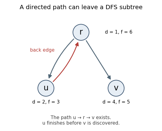
Past exam of the year 1 of the computer science course of the University of Oxford / 2018 / Functional programming, design and analysis of algorithms / 7 / b / ii / Solution by

Codex  0 2026-10-31

False. Use only the directed edge

u \to v

, but choose

v

first in the outer loop of depth-first search. It finishes before a second discovery tree starts at

u

d [v] = 1

f [v] = 2

d [u] = 3

f [u] = 4

. The edge supplies the required directed path and

f [u] > f [v]

, yet

d [u] > d [v]

. A path to an already black vertex need not put the two vertices into one discovery tree.

Past exam of the year 1 of the computer science course of the University of Oxford / 2018 / Functional programming, design and analysis of algorithms / 7 / b / i / Solution by

Codex  0 2026-10-31

False. Take two vertices

u, v

with both directed edges, and start depth-first search at

v

. The timestamps are

d [v] = 1

d [u] = 2

f [u] = 3

f [v] = 4

. There is an edge, hence a directed path, from

u

v

, but

f [u] < f [v]

. Reaching a gray ancestor does not make the ancestor finish first.

Past exam of the year 1 of the computer science course of the University of Oxford / 2018 / Functional programming, design and analysis of algorithms / 6 / c / iii / Solution by

Codex  0 2026-10-31

For

c \geq 2

, use largest-denomination-first greedy algorithm steps: for

i = n, n - 1, \dots, 1

, take

q_{i} = ⌊ r / c^{i} ⌋

coins and replace the residual amount

r

r - q_{i} c^{i}

. A target is representable exactly when it is divisible by

c

, because the smallest denomination is

c

, not one.

To prove optimality whenever the target is representable, observe that an optimum can have fewer than

c

coins of every denomination

c^{i}

with

i < n

: replacing

c

such coins by one

c^{i + 1}

coin preserves value and reduces the count by

c - 1

. After all such carrying, the coefficients of

c, c^{2}, \dots, c^{n - 1}

are the unique base-

c

digits of

v / c

, while the coefficient of

c^{n}

is the remaining quotient. Largest-first division produces exactly these coefficients. The greedy coin count is optimal, and can be computed with

O (n)

quotient/remainder operations without listing every coin.

For

c = 1

, distinct denominations permit only

n = 1

; then all coins have value one and the answer is

v

. This handles the printed positive-integer condition without silently assuming

c > 1

Past exam of the year 1 of the computer science course of the University of Oxford / 2018 / Functional programming, design and analysis of algorithms / 6 / c / ii / Solution by

Codex  0 2026-10-31

For the minimum coin change recurrence, initialize

C (0) = 0

and use

C (a) = 1 + min_{i : v_{i} \leq a} C (a - v_{i}),

where the minimum over no feasible predecessor is

\infty

and

1 + \infty = \infty

. Removing the last coin of an optimal representation proves the lower bound; appending the corresponding coin to an optimal predecessor proves attainability. $C (v)$ is the minimum number of coins, obtained in

O (n v)

time and

O (v)

space. Store one minimizing coin per amount if the actual coins are wanted.

Past exam of the year 1 of the computer science course of the University of Oxford / 2018 / Functional programming, design and analysis of algorithms / 6 / c / i / Solution by

Codex  0 2026-10-31

Use a Boolean dynamic programming state

R (a)

for whether amount

a

can be made exactly. Initialize

R (0) = True

and, for

a = 1, \dots, v

, compute

R (a) = ⋁_{i : v_{i} \leq a} R (a - v_{i}) .

An empty disjunction is false. Any nonempty representation ends in some coin; removing it gives one of the displayed predecessor states, and adding it back proves the converse. Return $R (v)$ . This takes

O (n v)

time and

O (v)

space for positive integer denominations and nonnegative integer target

v

, with unlimited coins of each type.