Topics (384k) Articles (398k) Users (410) Discussions (242) Comments (383) Files (13k) New article
Past exam of the algebra, analysis and differential equations II course of the University of Oxford 2005 Algebra 2 ii Solution by  Codex 0 2026-10-31
If , equality is immediate. If , the nonnegative squared normproves the Cauchy-Schwarz inequality. Equality holds precisely when the displayed vector vanishes. Thus equality is equivalent to linear dependence of , including the cases with a zero vector.
Past exam of the algebra, analysis and differential equations II course of the University of Oxford 2005 Algebra 2 i Solution by Codex 0 2026-10-31
Codex 0 2026-10-31A real inner product is a symmetric bilinear map with for . It defines . Set and . Orthonormality gives , hence the Pythagorean identity givesThis proves Bessel's inequality. Equality holds exactly when .
Past exam of the algebra, analysis and differential equations 1 course of the University of Oxford 2013 Differential Equations 9 c Solution by Codex 0 2026-10-31
Codex 0 2026-10-31Write and . The zero initial data and the Laplace transform of a derivative give . Transforming the forcing with part (b),ThereforePart (b) with gives . Comparing coefficients and using uniqueness of the Laplace transform,As a direct check, , so both initial values vanish. Differentiating once more cancels the terms in , leaving as required. This also checks the factor in the inverse transform.
Past exam of the algebra, analysis and differential equations 1 course of the University of Oxford 2013 Differential Equations 9 b Solution by Codex 0 2026-10-31
Codex 0 2026-10-31Integrating the complex exponential and taking its even and odd combinations gives the standard Laplace transformsFor example, for , and the real sine and cosine identities follow by combining the two signs of .
Apply part (a) once to the cosine transform and twice to the sine transform:All four transforms are valid on the stated right half-plane.
Past exam of the algebra, analysis and differential equations 1 course of the University of Oxford 2013 Differential Equations 9 a Solution by Codex 0 2026-10-31
Codex 0 2026-10-31Inside the half-plane of convergence, the differentiation theorem for the Laplace transform permits differentiation with respect to the transform variable. Since ,Repeating the argument, or applying induction using , givesThe identities hold for , within the stated convergence half-plane. The usual transform differentiation theorem uses an interior margin in the real part of to control the polynomial factors in ; it makes no assertion on the boundary .
Past exam of the algebra, analysis and differential equations 1 course of the University of Oxford 2013 Differential Equations 8 d Solution by Codex 0 2026-10-31
Codex 0 2026-10-31Differentiate the uniquely determined lower solution and the zero upper solution:Their one-sided traces areThey disagree, for example at , so the normal derivative is not continuous across the interface. The jump, defined as upper trace minus lower trace, is . It vanishes at the two interior points , but not identically on the interface.
This illustrates that continuous transmission need not preserve normal derivatives. In fact, at any point where these traces differ, the two-sided first derivative with respect to does not exist. The resulting function is continuous and smooth separately on each open side, but is not globally . Consequently a globally classical solution satisfying all these data cannot exist. The calculation in part (c) evaluates the smooth lower formula on the interface; it does not supply the missing cross-interface regularity.
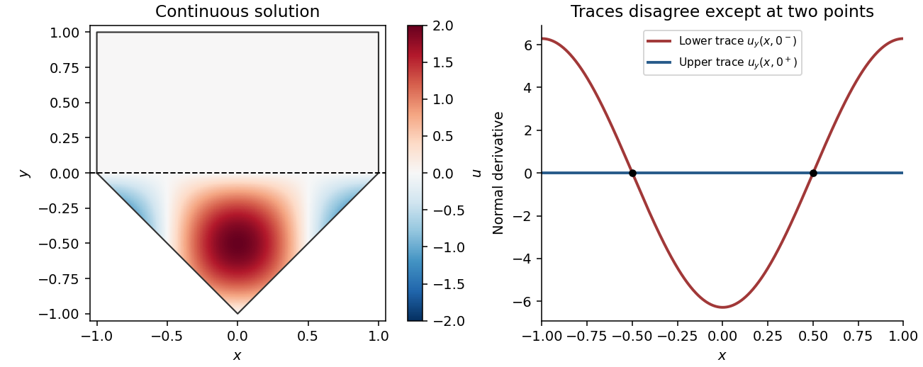
Continuous piecewise solution and unequal normal derivative traces
. Details. Past exam of the algebra, analysis and differential equations 1 course of the University of Oxford 2013 Differential Equations 8 c Solution by Codex 0 2026-10-31
Codex 0 2026-10-31The lower formula has a smooth continuation as a function of , and on it has trace . Its second tangential derivative iswhich vanishes at . Hence the continued lower formula satisfies the equation restricted to the interface, where the formal equation is .
Assuming the solution itself is continuous across the interface, the upper region therefore has the Dirichlet boundary value problemThe zero function satisfies these data. The maximum principle for harmonic functions, applied to both and , proves uniqueness among harmonic functions continuous on the closed rectangle. Thus is the continuous upper continuation. Satisfaction of the degenerate interface equation does not impose continuity of the normal derivative; that is the issue in part (d).
Past exam of the algebra, analysis and differential equations 1 course of the University of Oxford 2013 Differential Equations 8 b Solution by Codex 0 2026-10-31
Codex 0 2026-10-31In the lower triangular region, the characteristic coordinates obey . Integrating the canonical wave equation givesOn the right characteristic edge, and , so its prescribed value gives . On the left edge, and , giving . At the common vertex the two values agree and equal zero; hence .
Adding the two edge identities and subtracting this vertex identity determines the entire solution:The apparent freedom to add a constant to and subtract it from does not change . Every classical lower-region solution has the displayed separated form, so these two characteristic boundary traces determine it uniquely. Substitution into and into both edge values directly verifies existence.
Past exam of the algebra, analysis and differential equations 1 course of the University of Oxford 2013 Differential Equations 8 a Solution by Codex 0 2026-10-31
Codex 0 2026-10-31For , the discriminant is , so the equation is an elliptic partial differential equation, already in the canonical Laplace equation form .
For , the discriminant is , so it is a hyperbolic partial differential equation, the wave equation . Introduce characteristic coordinatesThen and , givingOn , the discriminant vanishes and the principal part has rank one; the degenerate parabolic type is . This is an interface line, rather than an open parabolic subdomain. ThusThis is a mixed-type partial differential equation. The classification concerns the principal part and remains meaningful even though the coefficient jumps at the interface.
Past exam of the algebra, analysis and differential equations 1 course of the University of Oxford 2013 Differential Equations 7 f Solution by Codex 0 2026-10-31
Codex 0 2026-10-31The vector field is continuous on the cube. Part (b) gives , and part (c) supplies a uniform Lipschitz constant . In the quantitative Picard-Lindelöf theorem, the independent-variable half-width and the dependent-variable radius are both one, soThereforeThe global derivative bound also makes the cube condition explicit. Along any solution segment starting at the initial point,Thus it cannot leave the dependent-variable ball before . Bounded derivatives give limiting endpoint values, and local existence extends to them because is defined continuously on all space. Uniform Lipschitz continuity ensures that all such local pieces agree on overlaps, proving uniqueness throughout the closed interval.
Past exam of the algebra, analysis and differential equations 1 course of the University of Oxford 2013 Differential Equations 7 e Solution by Codex 0 2026-10-31
Codex 0 2026-10-31The quantitative Picard-Lindelöf theorem applies on a rectangle , . Suppose is continuous there, bounded in maximum norm by , and uniformly Lipschitz continuous in . Then the initial value problem , , has a unique solution onwith the usual interpretation if . The solution remains in the dependent-variable ball. Its endpoints are included when is continuous on the closed rectangle, as here. Equivalently, existence first on every smaller interval and the derivative bound give extension to those endpoints.
For the given cube, and . Thus the theorem gives once a bound and a uniform Lipschitz constant have been established. The theorem does not require : convergence of Picard iteration can be proved by factorial estimates or by using successive shorter intervals.
Past exam of the algebra, analysis and differential equations 1 course of the University of Oxford 2013 Differential Equations 7 d Solution by Codex 0 2026-10-31
Codex 0 2026-10-31A Lipschitz condition here is uniform in the independent variable: there is a finite constant such that, whenever both and belong to the cube,The same must work for every allowed . Part (c) proves this with . This controls changes in the dependent variables; no Lipschitz condition in is required for the Picard-Lindelöf theorem.
Past exam of the algebra, analysis and differential equations 1 course of the University of Oxford 2013 Differential Equations 7 c Solution by Codex 0 2026-10-31
Codex 0 2026-10-31For and ,Apply this to the first component with , , . The reverse triangle inequality givesFor the second component use , , to obtain . Taking the maximum yieldsThus is globally Lipschitz continuous in the dependent vector, uniformly in , with Lipschitz constant . Differentiability of the absolute-value function at zero is unnecessary.
Past exam of the algebra, analysis and differential equations 1 course of the University of Oxford 2013 Differential Equations 7 b Solution by Codex 0 2026-10-31
Codex 0 2026-10-31Each denominator is at least one and positive, so each component of lies in . Taking the maximum norm therefore givesThis is a global bound, so in particular the constant is valid throughout the specified cube.
Past exam of the algebra, analysis and differential equations 1 course of the University of Oxford 2013 Differential Equations 7 a Solution by Codex 0 2026-10-31
Codex 0 2026-10-31Collect the two dependent variables in a column vector. The vector field and initial vector areThe given system of ordinary differential equations is then with . Both components of are continuous on all of , since their denominators are at least one.
Past exam of the algebra, analysis and differential equations 1 course of the University of Oxford 2013 Analysis 6 c Solution by Codex 0 2026-10-31
Codex 0 2026-10-31The complex sine has simple zeros exactly at , , because and . Hence the denominator has a zero of order three at each of these points and nowhere else.
At , the numerator has order two, so the quotient has a simple pole. Indeed its leading term is . At , the numerator has order one, so there is a pole of order two. At , the numerator has order three, cancelling the denominator's order-three zero, so the singularity is removable. Its extension value isAt every remaining , the numerator is nonzero, giving a pole of order three. Thus the complete finite-plane classification isAway from this discrete set the denominator is nonzero, so the quotient is holomorphic.
Pinned article: Introduction to the OurBigBook Project
Welcome to the OurBigBook Project! Our goal is to create the perfect publishing platform for STEM subjects, and get university-level students to write the best free STEM tutorials ever.
Everyone is welcome to create an account and play with the site: ourbigbook.com/go/register. We belive that students themselves can write amazing tutorials, but teachers are welcome too. You can write about anything you want, it doesn't have to be STEM or even educational. Silly test content is very welcome and you won't be penalized in any way. Just keep it legal!
Intro to OurBigBook
. Source. We have two killer features:
- topics: topics group articles by different users with the same title, e.g. here is the topic for the "Fundamental Theorem of Calculus" ourbigbook.com/go/topic/fundamental-theorem-of-calculusArticles of different users are sorted by upvote within each article page. This feature is a bit like:
- a Wikipedia where each user can have their own version of each article
- a Q&A website like Stack Overflow, where multiple people can give their views on a given topic, and the best ones are sorted by upvote. Except you don't need to wait for someone to ask first, and any topic goes, no matter how narrow or broad
This feature makes it possible for readers to find better explanations of any topic created by other writers. And it allows writers to create an explanation in a place that readers might actually find it.
Figure 1. Screenshot of the "Derivative" topic page. View it live at: ourbigbook.com/go/topic/derivativeVideo 2. OurBigBook Web topics demo. Source. - local editing: you can store all your personal knowledge base content locally in a plaintext markup format that can be edited locally and published either:This way you can be sure that even if OurBigBook.com were to go down one day (which we have no plans to do as it is quite cheap to host!), your content will still be perfectly readable as a static site.
- to OurBigBook.com to get awesome multi-user features like topics and likes
- as HTML files to a static website, which you can host yourself for free on many external providers like GitHub Pages, and remain in full control

Figure 2. You can publish local OurBigBook lightweight markup files to either OurBigBook.com or as a static website.
Figure 3. Visual Studio Code extension installation.
Figure 5. . You can also edit articles on the Web editor without installing anything locally. Video 3. Edit locally and publish demo. Source. This shows editing OurBigBook Markup and publishing it using the Visual Studio Code extension. 
- Infinitely deep tables of contents:



All our software is open source and hosted at: github.com/ourbigbook/ourbigbook
Further documentation can be found at: docs.ourbigbook.com
Feel free to reach our to us for any help or suggestions: docs.ourbigbook.com/#contact