For a second-order linear partial differential equation written $A{u}_{xx}+2B{u}_{xy}+C{u}_{yy}+\cdots =0$, the discriminant is $B^2-AC$. HereIt is positive exactly when $x\ne 0$, proving that the equation is a hyperbolic partial differential equation on each half-plane. At $x=0$ its principal part degenerates and it is not hyperbolic.

For $x,y>0$, the signs needed for the phase portrait follow directly from the factorizations:The coordinate axes are invariant sets. On $y=0$, the logistic differential equation $\dot{x}=x(1-x)$ directs positive states toward the boundary saddle point $(1,0)$. On $x=0$, $\dot{y}=2y$ directs positive states upward. At the three equilibria, use the local directions found in part (ii); interior sample trajectories near $(2,1)$ spiral clockwise inward.

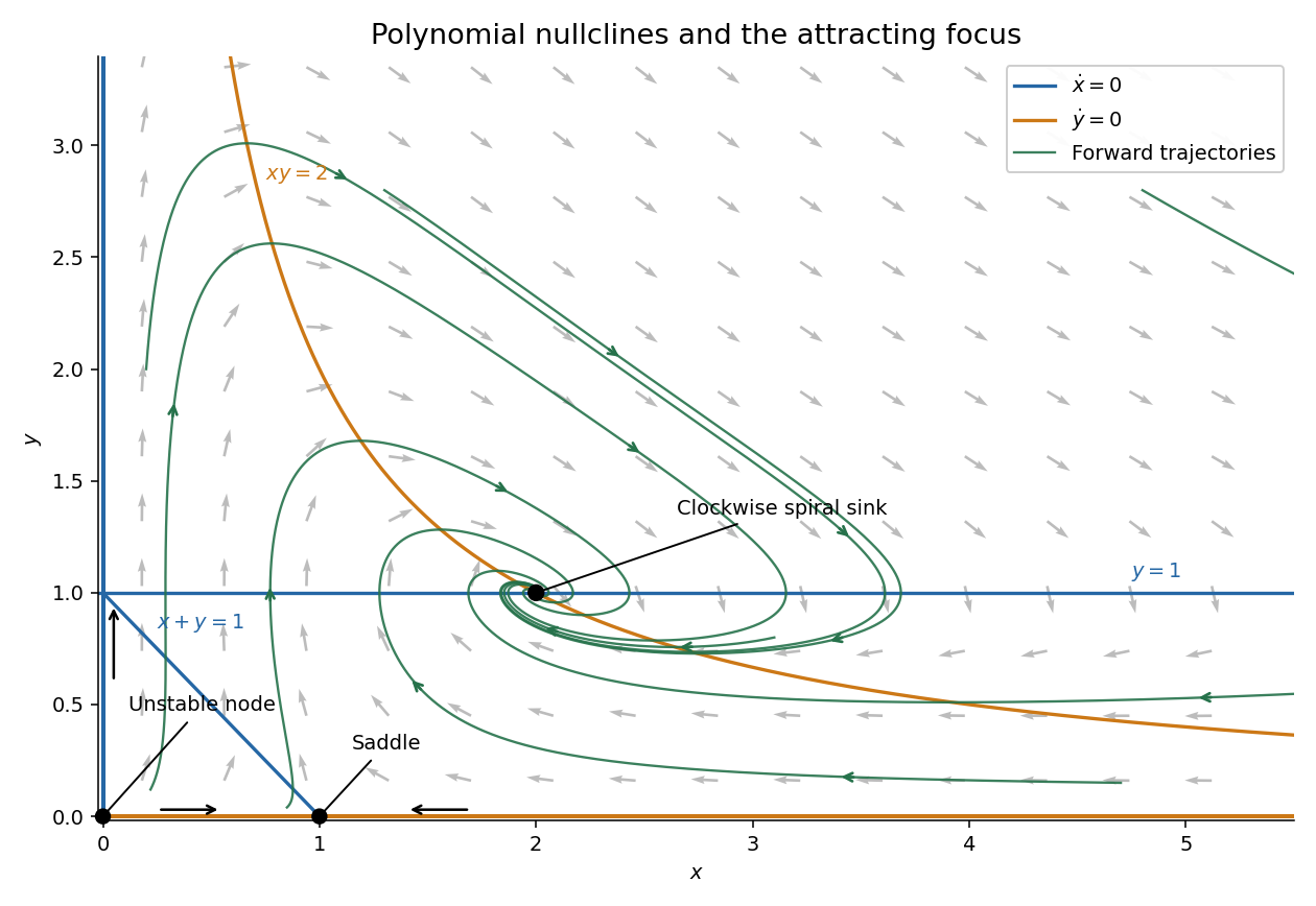
The nullclines prescribe where arrows become vertical or horizontal; they are generally not themselves trajectories. The image samples the vector field and several solutions, rather than assuming every nullcline is an invariant set.

Intersect the two nullcline families. The axes yield $(0,0)$ and $(1,0)$, and $y=1$ with $xy=2$ yields $(2,1)$. The possible remaining intersection would have $x+y=1$ and $xy=2$, requiring $x^2-x+2=0$, whose discriminant is $-7$. Hence there are no further real equilibria.

The Jacobian matrix isEvaluate it at each equilibrium:

All three are hyperbolic equilibria, so their classifications persist for the nonlinear system. Immediately to the right of $(2,1)$ on $y=1$, the velocity is vertically downward, showing that the attracting spiral turns clockwise.

Factor each component of the vector field. The horizontal-velocity nullclines and vertical-velocity nullclines are, respectively,The last curve is a hyperbola. In the nonnegative quadrant its branch is $y=2/x$ for $x>0$.

Translate the equilibrium to the origin by $z=(x-a,y-b{)}^T$. If the vector field is continuously differentiable, its first-order Taylor expansion isThe Jacobian matrix $M$ gives the linearization $\dot{z}=Mz$, whose general solution is $z(t)=e^{tM}z(0)$ using the matrix exponential. Its eigenvalues determine the exponential factors, while its eigenvectors and, when necessary, generalized eigenvectors determine their directions.

For distinct eigenvalues ${\lambda }_1,{\lambda }_2$ and corresponding eigenvectors $v_1,v_2$,For a real matrix with nonreal conjugate eigenvalues, choose conjugate coefficients to obtain real solutions. Equivalently, if $\lambda =a+ib$ and $v=p+iq$, a real pair of independent solutions isFor a repeated eigenvalue $\lambda$, there are two cases:

The factor $t$ in the second case is essential. These are exact solutions of the linearization; the remainder describes the error for the nonlinear differential equation. When no eigenvalue has zero real part, the hyperbolic equilibrium theory justifies the corresponding local qualitative classification. Zero real parts require additional nonlinear analysis.

An autonomous differential equation has no explicit dependence on the independent time variable: its vector field depends only on the current state. The two families of nullclines areOn the first family the horizontal velocity is zero; on the second the vertical velocity is zero. A critical point of a dynamical system is a state where both components vanish. It gives a constant solution, also called an equilibrium.

Regard the real skew-symmetric matrix as acting on ${\mathbb{C}}^n$. Its Hermitian adjoint is $A^{\ast }=A^T=-A$. Parts (i) and (iii) show that its eigenvalues are purely imaginary and its complex minimal polynomial has no repeated roots.

Since $A$ has real entries, nonreal eigenvalues occur in conjugate pairs. A nonzero pair has the form $i\alpha ,-i\alpha$, with $\alpha >0$, and contributes the real quadratic polynomialZero, if present, contributes one factor $x$. Hence the real minimal polynomial isThe product annihilates $A$ after complexification of a real vector space, so it also annihilates the original real linear map; no factor can be removed because each displayed complex root is an eigenvalue. This proves both the asserted form and its minimality. The case $A=0$ has $\epsilon =1$ and an empty product.

Proceed by induction on the dimension. For positive dimension, the fundamental theorem of algebra gives a root of the characteristic polynomial, hence a nonzero eigenvector $v$. Normalize it to have norm one. Its span is an invariant subspace, and part (ii) makes its orthogonal complement invariant too:The restriction of $T$ to the complement remains skew-adjoint, since the same inner product identity holds there. The induction hypothesis supplies an orthonormal eigenbasis for that smaller space. Adjoining $v$ gives an orthonormal eigenbasis for $V$.

The zero-dimensional base case is immediate. Thus $T$ is diagonalizable, indeed unitarily diagonalizable. This proves the finite-dimensional case of the spectral theorem for a skew-adjoint operator without assuming that distinct eigenvalues have multiplicity one.

Take $v\in U^{\perp }$ and $u\in U$. Because $U$ is an invariant subspace, $Tu\in U$. The adjoint operator relation yieldsThis holds for every $u\in U$, so $Tv\in U^{\perp }$. Therefore the orthogonal complement is also an invariant subspace.

Use the convention of part (a): the inner product is linear in its first argument. If $Tv=\lambda v$ with $v\ne 0$, the adjoint operator identity and $T^{\ast }=-T$ givePositive definiteness makes $⟨v,v⟩>0$, soThus every eigenvalue of a skew-adjoint operator is purely imaginary, including zero.

Writing $u={\sum }_i{u}_i{e}_i$ and $v={\sum }_i{v}_i{e}_i$, evaluation against the dual basis givesThis has codomain $\mathbb{C}$, not the printed $\mathbb{R}$. For a nonzero vector space, take $u=i{e}_1$ and $v=e_1$ to obtain $\varphi (u,v)=i$. Only the diagonal values $\varphi (v,v)$ must be real. The displayed formula defines the intended complex inner product.

It is linear in the first argument and conjugate-linear in the second:It has conjugate symmetry, since $\varphi (v,u)=\overline{\varphi (u,v)}$. Finally,with equality exactly when every coordinate vanishes, equivalently $v=0$. This proves positive definiteness. Since $\varphi (e_i,e_j)={\delta }_{ij}$, the original basis is orthonormal. This is the inner product determined by a basis.

Define the bidual evaluation map by evaluation:For fixed $v$, this is a linear functional of $\ell$, so it belongs to the double dual. It is also linear as a function of $v$. If $v\ne 0$, some coordinate of $v$ in a basis is nonzero, and the corresponding dual basis functional detects it. Hence $J(v)\ne 0$, proving injectivity.

The spaces $V,V^{\prime },V^{\prime \prime }$ all have the same finite dimension. Therefore an injective linear map $J:V\to V^{\prime \prime }$ is surjective, proving the required linear isomorphism.

This linear isomorphism is natural because evaluation requires no basis. More explicitly, for any linear map $A:V\to W$, its dual map satisfiesso $A^{\prime \prime }{J}_V=J_{W}A$.

The dual basis is the collection of linear functionals characterized byExplicitly, $e_i^{\prime }({\sum }_j{\alpha }_j{e}_j)={\alpha }_i$. Every linear functional $\ell \in V^{\prime }$ satisfies $\ell ={\sum }_i\ell (e_i)e_i^{\prime }$, proving that the displayed functionals span the dual space. Evaluating a zero linear combination at each $e_j$ makes all its coefficients zero, so they are also linearly independent. Thus they form a basis of $V^{\prime }$.

Suppose a single basis gives the diagonal matrices $D_S,D_T$. Entrywise multiplication gives $D_S{D}_T=D_T{D}_S$. If $P$ is the change-of-basis matrix, thenThus simultaneous diagonalization implies commutation.

On each nonzero eigenspace $V_{\lambda }$, the restricted linear map $S_{\lambda }=S{|}_{V_{\lambda }}$ is diagonalizable. Indeed $m_S(S_{\lambda })=0$, so the minimal polynomial of $S_{\lambda }$ divides $m_S$. A divisor of a product of distinct linear polynomials has the same property, proving the diagonalizable restriction lemma.

Choose a basis of $S_{\lambda }$-eigenvectors in each $V_{\lambda }$. Every chosen vector is simultaneously a $T$-eigenvector, with eigenvalue $\lambda$. The direct sum in part (ii) shows that joining these bases gives a basis of $V$. Therefore $S$ and $T$ have a common eigenbasis, which is exactly simultaneous diagonalization.

For $v\in V_{\lambda }$, use commutation to obtainThus $Sv\in V_{\lambda }$, proving that every $T$-eigenspace is an $S$-invariant subspace. This does not assert that an arbitrary eigenvector of $T$ is already an eigenvector of $S$.

Since $T$ is diagonalizable, its minimal polynomial is ${\prod }_{j=1}^r(x-{\lambda }_j)$ with distinct eigenvalues ${\lambda }_j$ in the field. Apply the primary decomposition theorem for linear maps:For a scalar that is not an eigenvalue, the associated eigenspace is zero, so the sum indexed by the whole field has only finitely many nonzero summands. The eigenspaces need not be one-dimensional.

The primary decomposition theorem for linear maps states that ifwith distinct monic irreducible polynomials $p_j$, thenEach summand is a $T$-invariant subspace. More generally the same direct sum conclusion holds for any factorization of an annihilating polynomial into pairwise coprime polynomials, using the corresponding kernels. The underlying mechanism is the Bézout's identity for polynomials, which separates the mutually coprime factors.

In the finite field ${\mathbb{F}}_2$, the matrix becomesOn the first two coordinate vectors it is a nonzero nilpotent Jordan block of size two, and on the last it is the identity map. ConsequentlyThe repeated zero root prevents diagonalizability. Directly, the only possible eigenvalues are zero and one, so diagonalizability would imply $A^2=A$, whereas the displayed off-diagonal entry disappears on squaring.

In the finite field ${\mathbb{F}}_3$, reduce the characteristic polynomial to $(x-1{)}^3$. For $B=A-I$, reduction of the entries givesHenceIts repeated linear polynomial prevents diagonalizability. Equivalently, a diagonalizable map with only the eigenvalue one would have to be $I$, and this matrix is not $I$.