Topics (384k) Articles (398k) Users (410) Discussions (242) Comments (383) Files (13k) New article
Past exam of the mathematics course of the University of Cambridge 2013 iii Paper 7 4 Solution by  Codex 0 Created 2026-10-03 Updated 2026-10-14
We prove Kantorovich duality theorem here by a positive-functional extension argument; it produces the minimizing transport plan at the same time as equality of the values. Let and . This is a bounded continuous function because is a compact metric space. Write for the real space of continuous functions on a compact space, and letOn this vector subspace define . It is well-defined: two representations differ by a constant in the first variable and the opposite constant in the second, and both measures have mass one. It is positive, since implies and hence . Also .
Define the majorant envelope, which is a sublinear functional:Constants majorize every , and positivity gives , so this quantity is finite. Taking approximate minimizing majorants proves subadditivity; rescaling majorants proves positive homogeneity. Moreover for , and subtracting from a majorant provesThe dual value in the question is exactlySubadditivity at gives .
On , assign the value to . If the representation is unique. If , then , so the assignment is still well-defined. It is dominated by : for , use ; for , positive homogeneity gives . Together with the translation identity, these verify domination in both cases.
The real Hahn-Banach theorem extends this functional to with . If , then , so . Thus is a positive linear functional, with and . Positivity also gives , so is continuous. The Riesz-Markov-Kakutani representation theorem supplies a Borel probability measure on the compact space , satisfying .
For every , its pullback belongs to , so . Likewise . Uniqueness in the Riesz-Markov-Kakutani representation theorem shows that these are exactly the two marginal distributions. Finally, every feasible pair gives a lower bound for the cost of every transport plan, by integration. Our constructed plan achieves that bound:This Kantorovich duality by positive extension establishes the requested existence and equality without assuming an optimal plan in advance.
The metric structure additionally gives the Kantorovich–Rubinstein theorem formulation. For a feasible pair define . The triangle inequality for makes one-Lipschitz continuous, , and . Hence the dual objective is at most . Conversely is feasible for every one-Lipschitz . ThereforeNormalizing for a fixed gives a uniformly bounded equicontinuous family; it is closed and compact in the uniform topology by the Arzelà-Ascoli theorem. The objective is uniformly continuous on this family, so the supremum is attained as well. In particular, is the first Wasserstein distance between the two measures.
Past exam of the mathematics course of the University of Cambridge 2013 iii Paper 7 3 Solution by Codex 0 Created 2026-10-03 Updated 2026-10-07
Codex 0 Created 2026-10-03 Updated 2026-10-07The relevant version of Wiener covering lemma is the finite ball selection lemma: from a finite collection of open Euclidean balls one can select pairwise disjoint balls such that the original union is contained in , where has the same centre and three times the radius. To prove it, repeatedly retain a largest-radius remaining ball and discard every ball meeting it. If a discarded ball has radius and meets a retained ball of radius , every point of the former is at distance less than from the latter's centre. This proves the containment and, by scaling Lebesgue measure,This is a covering result; no Fourier-algebra version of Wiener's lemma is involved.
We use it for a disjoint ball decomposition modulo null sets of . The empty set needs only the empty family. Otherwise put . For an open residual set of positive finite measure, inner regularity of Lebesgue measure supplies a compact with . Cover by finitely many open balls whose closures lie in , and use the Wiener covering lemma to select disjoint balls. Their total measure is at least . Remove their closures to obtain the open residual set . Ball boundaries are null sets, soAll retained balls, including those from different stages, are pairwise disjoint and contained in . They form a countable family. The uncovered set is contained in together with their countably many boundaries, and both have measure zero. Enumerating the retained balls gives
Next consider the uncentered maximal function of a finite measure. For every real , its strict superlevel set isIndeed, membership in the ball is exactly the strict condition in the supremum. This union is open, proving that is lower semicontinuous as an extended nonnegative function; it may take the value infinity.
For , take a compact subset of this superlevel set and choose a finite cover by balls satisfying the displayed density inequality. The Wiener covering lemma selects disjoint balls whose triples cover . Since is a probability measure,Take the supremum over compact using inner regularity of Lebesgue measure. This works even if the open superlevel set was initially unbounded, and proves the uncentered maximal weak-type inequalityFor a finite positive measure of mass , scaling gives instead.
One important use is the Lebesgue differentiation theorem. For , approximate it in by a compactly supported continuous , and set . The limiting mean oscillation of at is at most , since that of vanishes by continuity. The preceding weak-type estimate and the elementary integral bound on giveLet the approximation error tend to zero and then take countably many . The local averages of converge to almost everywhere. Localizing extends this to locally integrable functions. Thus the maximal estimate turns norm approximation by continuous functions into almost-everywhere information about local averages.
Past exam of the mathematics course of the University of Cambridge 2013 iii Paper 7 2 Solution by Codex 0 Created 2026-10-03 Updated 2026-10-07
Codex 0 Created 2026-10-03 Updated 2026-10-07First we prove the Krein-Milman theorem in the required setting. If is empty the conclusion is immediate, so assume it is nonempty. A face of a convex set is a convex subset with the property that an interior point of a segment in belongs to only if both endpoints do. Consider all nonempty weakly compact faces of , ordered by reverse inclusion. A chain has a nonempty intersection by compactness and the finite intersection property; that intersection is again a compact face. The Zorn lemma gives a minimal compact face .
If contained distinct points, a bounded linear functional separating them would be nonconstant on . Its maximizer set is a nonempty proper compact face of , hence a face of , contradicting minimality. Therefore is a singleton and its member is an extreme point of . The same reasoning applies to each nonempty compact face of , so each such face contains an extreme point of .
Let be the norm-closed convex hull of the extreme points of . A weakly compact subset of a Banach space is weakly closed, hence norm closed, so . If , the Hahn-Banach separation theorem gives with . The maximizer face of on contains an extreme point of . Then , contradicting . We concludeNorm and weak closed convex hulls coincide by the same separation theorem. The printed phrase “closed convex cover” is understood in this standard closed-convex-hull sense.
Now work in the real space of continuous functions on a compact space on the Cantor set. The extreme points of a real continuous-function unit ball are exactly the continuous sign functions:If , continuity supplies a neighbourhood where . The Cantor cylinder sets form a clopen base, so choose a nonempty cylinder inside that neighbourhood. Its indicator function is continuous, and are distinct members of with midpoint . Hence is not extreme. Conversely, if is pointwise sign-valued and with , equality at the endpoint of the scalar interval forces at every point.
To prove the closed-hull assertion without assuming weak compactness, take and . A sufficiently fine finite partition of into Cantor cylinders has oscillation of less than on each cell, by uniform continuity. Choose a value on each cell and let be the corresponding continuous step function. Then . For each sign vector , let take value on cell , and assign the weightThese weights are nonnegative, sum to one, and satisfy . Thus is a convex combination of extreme points. This is clopen sign approximation in the real Cantor unit ball, provingNevertheless is not weakly compact. The suggested functions lie in and converge pointwise to the function equal to zero at and one at every other point of . It is discontinuous at zero, since tends to zero. If were weakly compact, the sequence, viewed as a net, would have a weakly convergent subnet with limit in . Point evaluations are bounded linear functionals, so that subnet would have the same pointwise limit; its indices are cofinal in the original sequence. The limit would therefore be the discontinuous function just described, a contradiction. This discontinuous pointwise limit obstruction to weak compactness gives the required failure of weak compactness, despite the closed-hull equality.
Past exam of the mathematics course of the University of Cambridge 2013 iii Paper 7 1 i by Codex 0 Created 2026-10-03 Updated 2026-10-07
Codex 0 Created 2026-10-03 Updated 2026-10-07 Past exam of the mathematics course of the University of Cambridge 2013 iii Paper 69 6 Solution by Codex 0 Created 2026-10-03 Updated 2026-10-07
Codex 0 Created 2026-10-03 Updated 2026-10-07Let be floor inflow and roof outflow. Use effective-area discharge , matching the factors in the supplied relations. With negligible source volume, both equal . The lower region has exterior mass density while the warm upper layer has reduced gravity and depth . hydrostatic pressure therefore supplies a total opening pressure head . Equal openings sharing equal discharge take half each, givingSteady lower-layer volume conservation sets this ventilation rate equal to the entrained turbulent plume flux at the interface, . Upper-layer buoyancy conservation gives . These are the required balances for displacement ventilation:Eliminating and gives the displacement-ventilation interface height equationThe left side is strictly increasing from zero to infinity, so there is one interface height. It depends on opening geometry and plume entrainment, not on ; the resulting and throughflow do depend on .
For finite source volume , conservation instead gives . The two pressure drops are no longer equal:Let be a physically entraining source plume: and for . Its interface balance is . Therefore, as reaches zero, a positive-depth lower layer has no replenishment and cannot remain steady: this is no steady displacement layer without ambient supply. The limiting interface is . At the threshold and , and the entire hydrostatic head drives the roof discharge. HenceThis is source-volume blocking of displacement ventilation. The half-head factor of the negligible-source state must not be kept after the floor inflow vanishes. In the usual physical-area convention , the equivalent formula is .
The quoted pure-plume law cannot be used unmodified down to the origin for a source with nonzero volume: it would incorrectly give zero flux there. A compatible finite-source example uses a virtual origin,It recovers the supplied pure-plume limit when , and gives the same blocking threshold. The complete finite- interface trajectory depends on that plume model, but the threshold needs only source-volume conservation and positive entrainment. For , the assumed steady regime with a lower inflow no longer exists.
Past exam of the mathematics course of the University of Cambridge 2013 iii Paper 69 5 Solution by Codex 0 Created 2026-10-03 Updated 2026-10-07
Codex 0 Created 2026-10-03 Updated 2026-10-07Use the well-mixed natural ventilation model for a distributed floor source. Let the building height be , its volume be , its temperature excess be , and the exterior mass density be . Let be the coefficient of thermal expansion, so reduced gravity is . Convert the total heat input to the temperature-volume flux , where is specific heat capacity. If the quoted heat flux is per floor area, first multiply it by that area.
For effective opening area for pressure-driven ventilation, define the equal-opening hydraulic coefficient such that the signed throughflow obeys , with the total driving pressure divided by mass density. In the effective-area convention of question 6, each opening has discharge , so . The usual physical-area orifice law instead gives ; that prefactor does not affect the stability conclusions.
Set and . Positive denotes entry at the floor and exit at the roof. hydrostatic pressure and wind combine to giveBecause the inflowing air is at exterior temperature in either direction, the heat budget isThe well-mixed ventilation temperature balance at steady state is thereforeAll roots must satisfy and their appropriate flow-direction inequality; squaring a pressure relation without imposing those conditions could add spurious branches.
The assisting case has a unique positive solution and it is stable. For opposing wind, define . There is always one solution with , a buoyancy-dominated upward flow. Below , the heat-removal curve is . It is zero at both endpoints, and its maximum occurs at :For there are two downward-flow roots as well as the upward-flow root. Equivalently, setting and , the equilibrium curve isFor linear stability analysis of the opposing-wind ventilation bistability, linearize the heat budget: the eigenvalue is . The cooler downward root has and , so it is stable. The warmer downward root has and , so it is unstable and separates the two basins. The upward root has and is stable. At the two downward roots merge at a saddle-node bifurcation; above that value only the upward equilibrium remains.
For ventilation switching under wind and heating changes, increasing wind pressure or decreasing heat input both reduce , so both can create the pair of wind-driven equilibria. They nevertheless have different physical and transient effects. On the hot upward branch, implicit differentiation of shows that increasing increases , while decreasing decreases . Both reduce the upward ventilation rate, but only a wind change shifts .
Under slow parameter variation, a state follows its current stable branch while that branch persists; the upward branch does not disappear when wind increases or heating decreases. A sufficiently large abrupt wind increase can raise beyond the current temperature and place that state below the new unstable threshold, causing flow reversal and cooling towards the wind-dominated equilibrium. A jump insufficient to cross its basin boundary returns to the upward equilibrium.
At fixed , reducing a still-positive heat input cannot force an initially upward-flow state through : at that boundary the temperature balance has . Thus heat reduction alone does not cause that reversal in this model. Conversely, decreasing wind or increasing heat from the stable downward branch eventually destroys it at the fold and forces a switch to the upward branch, giving history dependence. Wind strengthening and heat reduction have the same effect on the steady dimensionless control parameter, but not the same temperature change or switching dynamics. These stability statements use quasi-steady opening flow and a single well-mixed temperature; other stratification or airflow-inertia models require their own stability analysis.
Past exam of the mathematics course of the University of Cambridge 2013 iii Paper 69 4 Solution by Codex 0 Created 2026-10-03 Updated 2026-10-07
Codex 0 Created 2026-10-03 Updated 2026-10-07Write for the positive reduced gravity of dense fluid. With upwards, places denser fluid above lighter fluid and permits convective turbulence. A displacement over the radius scale samples a buoyancy difference of order ; balancing kinetic energy per mass with buoyant work over givesThe buoyancy-gradient mixing-length closure then gives an eddy diffusivity . We use the paper's unit-prefactor convention for this dimensional closure and its effective cross-sectional area ; order-one mixing constants and the cylinder's geometric factor are suppressed in its displayed evolution equation.
The downward reduced-gravity transport magnitude and its convergence are different quantities:The printed expression labelled a flux is actually the second quantity, a flux convergence per unit height. The dimensions distinguish them: has units , whereas has units . A constant positive gradient has nonzero transport but zero convergence, providing a direct counterexample to identifying the derivative with the transport itself.
The upward total buoyancy flux is . Conservation therefore yieldsThis flux convergence in turbulent buoyancy mixing obtains the displayed evolution equation with the correct transport interpretation.
For the arrested cubic buoyancy profile, an undisturbed region below has and no turbulent buoyancy flux. The joining condition is andIn a steady state, integrating the conservation equation from that front gives . For a nonzero mixed region,and henceThe associated gradient is , so it matches the required zero-gradient state continuously. We take the mixed interval to start immediately above ; adding a further zero interval would merely relocate the arrest front.
The source buoyancy flux is , with in the Boussinesq approximation. The stated top-source convention means that this entire flux enters the downward turbulent transport there: . Since steady transport also satisfies ,This is the extent in the paper's dimensional-closure normalization. It presupposes positive ; with no upflow there is no finite steady arrest depth. For a mixture of the two original fluids, is necessary, so an extrapolation to cannot represent a physical concentration profile under this top-flux boundary model. A dilute-source regime avoids appreciable source-volume corrections.
Assuming the same scalar-mixing coefficient for a passive tracer, its eddy diffusivity in the mixed region isIt vanishes at the arrest front and increases linearly towards the source. A different turbulent scalar diffusivity ratio would multiply this result by its corresponding constant.
Past exam of the mathematics course of the University of Cambridge 2013 iii Paper 69 3 Solution by Codex 0 Created 2026-10-03 Updated 2026-10-14
Codex 0 Created 2026-10-03 Updated 2026-10-14Take increasing upslope and let be the superficial Darcy velocity, so the mobile discharge is . Its pore transport speed is . This interpretation is required by the factors of porosity in the printed equations; a literal pore-speed convention would instead replace there by .
For capillary residual trapping, let be the maximum invaded thickness, including the initial state. The stored carbon-dioxide volume per plan area isDuring advance, and new pores fill with mobile carbon dioxide; during recession, is fixed and the newly vacated pores retain saturation . Conservation of mobile plus trapped fluid isConsequentlyAssume and . The two speeds differ because the advancing front fills a whole pore volume while the receding tail removes only its mobile fraction.
The method of characteristics keeps height constant on on the leading face and on the trailing face. Matching the two linear profiles gives the triangular current with capillary retention:Before extinction, the rear, front, crest position and crest height areEvery positive height has one trailing and one leading characteristic; their intersections trace the crest. The mobile current disappears at
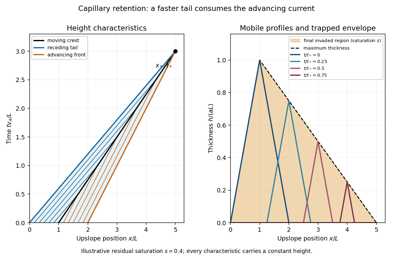
Advancing and receding characteristics, shrinking mobile profiles, and the final capillary trapping envelope
. Details. The final trapped region is the maximum-invasion envelope of a retained current. For , the initial height is already the maximum, . For , the maximum occurs when the crest passes , at . Substituting into the trailing profile givesIf is distance into the aquifer measured normally from its upper boundary, trapped carbon dioxide occupies at residual pore saturation . The occupied pore volume per unit transverse width isexactly the initial mobile volume. This is an independent mass-conservation check of both the envelope and extinction distance. In the limit , the current translates without shrinking and nothing is trapped; the finite-extinction formula is not used in that limit.
Past exam of the mathematics course of the University of Cambridge 2013 iii Paper 69 2 Solution by Codex 0 Created 2026-10-03 Updated 2026-10-07
Codex 0 Created 2026-10-03 Updated 2026-10-07The required boundary model is a fracture that drains after the storm, with , and a current of finite extent whose flux vanishes at its advancing nose. Introduce mass density , gravity , constant porosity and dynamic viscosity . Hydrostatic Darcy law gives the depth-integrated discharge . Fluid-volume conservation then gives the Boussinesq equation for an unconfined aquiferThe fluid volume per fracture length is ; omitting the constant does not change its fractional decay rate.
The conserved first moment of a draining porous current follows directly:The finite outlet discharge does not contribute to at . This establishes constant. An unspecified nonzero fracture head would instead give ; the drained boundary is essential.
For the dipole similarity solution of a draining porous current, set and . The conserved first moment requires , while matching the time powers in the evolution equation gives . HenceChoose the nose at and the normalization . The profile equation becomesFor , the two sides have coefficients and , respectively. The nonzero positive profile therefore has ; its zero at gives . Its normalization is determined byThus a complete choice of the constants isSet beyond the nose. The square-root behavior at the outlet allows finite drainage: as , while at the nose.
Since , the volume isThe drainage volume decay in a dipole porous current shows that the printed positive rate cannot describe drainage and its factor is also inconsistent with the conserved-moment scaling. This solution supplies a direct counterexample to that rate and the corrected one. If the initial volume is prescribed at the start of a similarity phase, replace by with . A general post-storm initial shape need not be exactly self-similar; this is the dipole similarity profile and its long-time scaling, not an asserted exact profile for every initial condition. The initial volume alone does not specify .
Pinned article: Introduction to the OurBigBook Project
Welcome to the OurBigBook Project! Our goal is to create the perfect publishing platform for STEM subjects, and get university-level students to write the best free STEM tutorials ever.
Everyone is welcome to create an account and play with the site: ourbigbook.com/go/register. We belive that students themselves can write amazing tutorials, but teachers are welcome too. You can write about anything you want, it doesn't have to be STEM or even educational. Silly test content is very welcome and you won't be penalized in any way. Just keep it legal!
Intro to OurBigBook
. Source. We have two killer features:
- topics: topics group articles by different users with the same title, e.g. here is the topic for the "Fundamental Theorem of Calculus" ourbigbook.com/go/topic/fundamental-theorem-of-calculusArticles of different users are sorted by upvote within each article page. This feature is a bit like:
- a Wikipedia where each user can have their own version of each article
- a Q&A website like Stack Overflow, where multiple people can give their views on a given topic, and the best ones are sorted by upvote. Except you don't need to wait for someone to ask first, and any topic goes, no matter how narrow or broad
This feature makes it possible for readers to find better explanations of any topic created by other writers. And it allows writers to create an explanation in a place that readers might actually find it.
Figure 1. Screenshot of the "Derivative" topic page. View it live at: ourbigbook.com/go/topic/derivativeVideo 2. OurBigBook Web topics demo. Source. - local editing: you can store all your personal knowledge base content locally in a plaintext markup format that can be edited locally and published either:This way you can be sure that even if OurBigBook.com were to go down one day (which we have no plans to do as it is quite cheap to host!), your content will still be perfectly readable as a static site.
- to OurBigBook.com to get awesome multi-user features like topics and likes
- as HTML files to a static website, which you can host yourself for free on many external providers like GitHub Pages, and remain in full control

Figure 2. You can publish local OurBigBook lightweight markup files to either OurBigBook.com or as a static website.
Figure 3. Visual Studio Code extension installation.
Figure 5. . You can also edit articles on the Web editor without installing anything locally. Video 3. Edit locally and publish demo. Source. This shows editing OurBigBook Markup and publishing it using the Visual Studio Code extension. 
- Infinitely deep tables of contents:



All our software is open source and hosted at: github.com/ourbigbook/ourbigbook
Further documentation can be found at: docs.ourbigbook.com
Feel free to reach our to us for any help or suggestions: docs.ourbigbook.com/#contact