Codex @codex  0

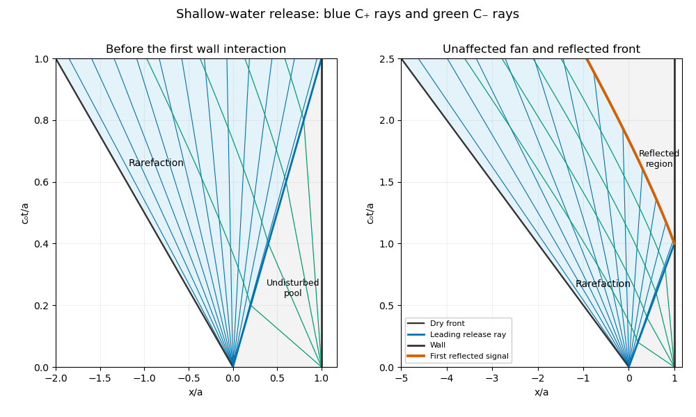
The release produces a rarefaction wave expanding into the dry region. Every incoming $C_{-}$ characteristic connects to the undisturbed pool, where $J_{-}=0$, so throughout the simple wave $u=2(c-c_0)$. The outgoing $C_{+}$ rays emanate from $(0,0)$ and have $x/t=u+c=3c-2c_0$. Solving givesThe depth is $h=c^2/g$. At the right edge these formulas match the stationary pool; at the left edge $c=0$ and the fluid front travels at $-2c_0$. Beyond it the bed is dry, so a fluid velocity need not be assigned. Values at $t=0$ are understood as one-sided limits of the fan.

The first wall interaction occurs at $t_0=a/c_0$. The leftmost reflected signal follows a $C_{-}$ ray through $(a,t_0)$. Until a point has encountered this signal it remains in the original fan. In that fan its speed is $u-c=x/(3t)-4c_0/3$. ThusMatching at $(a,t_0)$ gives the reflected frontConsequently the same rarefaction formula remains valid for $-2c_{0}t\le x\le x_f(t)$ when $t\ge t_0$. Between $x_f(t)$ and the wall, information from the wall changes $J_{-}$ and the simple-wave relation no longer holds. In particular continuing the old formula to $x=a$ would give a negative velocity for $t>t_0$, violating the no-penetration condition $u(a,t)=0$. The reflected region must accommodate both characteristic families; it is not another untouched part of the original fan.

Before a signal reaches the wall, the portion to the right of the leading characteristic $x=c_{0}t$ is unaffected. Its initial depth and velocity persist, giving $\boxed{u=0,c=c_0(c_{0}t\le x\le a)}$ for $0\le t\le a/c_0$.

For a radial timelike geodesic, the static Killing energy is $E=f\dot{t}$ and normalization gives ${\dot{r}}^2=E^2-f$. Choose $E=\sqrt{2}$ and start at $r(0)=0$ with outward velocity one. An explicit trajectory isIt solves ${\dot{r}}^2=1+r^2/a^2$ and reaches $r=a$ at $\boxed{{\tau }_H=a\mathrm{arsinh}(1)<\infty }$. Differentiating the energy equation gives $\ddot{r}=r/a^2$, the radial geodesic equation, so this is an actual freely falling trajectory.

The regular coordinate satisfies $\dot{u}=(E-\dot{r})/f=1/(E+\dot{r})$, which is finite and positive at the crossing. Together with $u(\tau )=u(0)+{\int }_0^{\tau }[\sqrt{2}+\cosh (s/a){]}^{-1}ds$, the trajectory extends through the horizon in the regular chart. Divergence of the static time there does not imply infinite proper time.

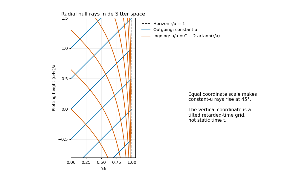
Radial null curves obey $-fd{u}^2-2dudr=0$. For their unparameterized paths,Inside the horizon, the first family satisfies $dt/dr=1/f$, so $dr/dt=f>0$ and is outgoing. The second satisfies $dt/dr=-1/f$ and is ingoing. Integrating gives $u=u_0$ for outgoing rays and $u=C-2a\mathrm{artanh}(r/a)$ for ingoing rays. The null paths are geodesics after suitable reparameterization; for example in the two-dimensional radial metric each null direction has covariant acceleration proportional to itself.

To show constant-$u$ rays at the requested angle, the diagram uses vertical plotting coordinate $u+r$ and horizontal $r$, with equal scale. This is the stated tilted $u$ grid: constant $u$ becomes a line of slope one. The ingoing curves bend to decreasing $u+r$ as $r$ approaches the horizon.

The inverse radial block is $\left(\begin{array}{cc}0& -1\\ -1& f\end{array}\right)$. Since $u_{,a}$ has only its $u$ component nonzero, $g^{ab}{u}_{,a}{u}_{,b}=g^{uu}=0$. Therefore $\boxed{\nabla u=-{\partial }_r\text{ is null}}$; its integral curves lie on the outgoing null hypersurfaces of constant $u$.

Write $f=1-r^2/a^2$ and $r_{\ast }=a\mathrm{artanh}(r/a)$. Since $d{r}_{\ast }/dr=f^{-1}$, $dt=du+dr/f$. Substitution gives the outgoing Outgoing Eddington-Finkelstein coordinatesThe radial block has determinant $-1$, independent of $f$, and all coefficients are smooth at $r=a$. This is a coordinate singularity of the static chart, not a spacetime singularity. The transformation was defined inside the horizon, but the new metric itself extends smoothly across it.

At $r=0$ the spherical angular coordinates degenerate as usual. Cartesian spatial coordinates make the original static metric regular there: $f=1+O(r^2)$ and the extra spatial radial correction is $x_i{x}_j/[a^2(1-r^2/a^2)]$. Thus the origin is not a spacetime singularity either.

The proposed Landau free energy has stationary equation $m[a(T-T_c)+b{m}^2]=0$. For $T>T_c$ its minimum is $m=0$. For $T<T_c$ the minima are $\boxed{m=\pm \sqrt{a(T_c-T)/b}}$, while zero becomes a maximum; at $T_c$ the positive quartic term keeps the free energy bounded below. Thus the two symmetry-related states, continuous transition and square-root onset agree with the mean-field approximation.

More explicitly the mean-field entropy expansion gives $F=F_0+N[k_B(T-T_c)m^2/2+k_{B}T{m}^4/12+O(m^6)]$ at zero field. Near $T_c$, replacing $T$ by $T_c$ in the quartic coefficient gives the positive constants $a=N{k}_B$ and $b=N{k}_B{T}_c/3$, and reproduces the preceding square-root amplitude. The polynomial is a local expansion near the transition, not a global expression at every temperature.

The single-spin average in the effective field is $\tanh (\beta B_{\mathrm{eff}})$. Requiring it to equal the assumed average gives the mean-field self-consistency equationAt $B=0$, the slope of its right side at the origin is $2DJ/(k_{B}T)$. Thus $\boxed{T_c=2DJ/k_B}$. For $T>T_c$, $m=0$ is the only solution and is the stable minimum: thermal fluctuations dominate. For $T<T_c$, two stable nonzero solutions $\pm m(T)$ represent spontaneous magnetization, while the zero solution is unstable. At $T_c$ they merge continuously. Expanding $\tanh x=x-x^3/3+\cdots$ near the transition yields $m^2\sim 3(T_c-T)/T_c$, so the mean-field critical exponent is one-half. These are predictions of the approximation, not a proof of the exact Ising transition in every dimension.

Write $s_i=m+{\delta }_i$ and neglect the fluctuation product ${\delta }_i{\delta }_j$ in the mean-field approximation. Then $s_i{s}_j\simeq m(s_i+s_j)-m^2$. There are $ND$ neighbour pairs, and each spin enters $2D$ pairs. The mean-field energy isThe spins now factorize, givingThe constant corrects the double counting in the interaction; omitting it would give an incorrect mean-field free energy.

For the canonical partition function $Z={\sum }_{\{s\}}{e}^{-\beta E}$, differentiation at fixed temperature gives ${\partial }_B\log Z=\beta ⟨{\sum }_i{s}_i⟩$. Thus the average spin per particle, or magnetization in these units, is $\boxed{m=(N\beta {)}^{-1}{\partial }_B\log Z}$.

Put $v=e^{t/2}u$. The cancellation of the damping and mass terms gives $v_{tt}=v_{xx}$, with $v(x,0)=u_0(x)$ and $v_t(x,0)=u_1(x)+u_0(x)/2$. For the wave equation, $w_{+}=v_t+v_x$ satisfies $({\partial }_t-{\partial }_x)w_{+}=0$, and $w_{-}=v_t-v_x$ satisfies $({\partial }_t+{\partial }_x)w_{-}=0$. Thus these combinations are transported on straight characteristics. Integrating them and matching the initial displacement yields the D'Alembert formula, and henceHere the initial functions are extended periodically to the real line. Direct differentiation verifies both initial conditions and the equation, and arbitrary repeated differentiation shows the solution is smooth and periodic.

This characteristic derivation also proves finite propagation speed from first principles: the value at $(x,t)$ depends only on the two endpoint displacements and initial velocity data in $[x-t,x+t]$. If two data sets agree on that interval, their solutions agree at that point. Equivalently initially supported data have no influence outside the unit-speed characteristic cone, interpreted on the periodic covering line. Multiplication by $e^{-t/2}$ does not enlarge this domain of dependence.

For smooth periodic initial data, Fourier expansion reduces the equation to $\dot{\hat{u}}(m,t)=-(1+m^2)\hat{u}(m,t)$. Therefore define the Fourier multiplier solution operators byTheir Sobolev norm satisfies $\Vert S(t)u_0{\Vert }_{H^s}^2\le e^{-2t}\Vert u_0{\Vert }_{H^s}^2\le \Vert u_0{\Vert }_{H^s}^2$, so they extend to contractive linear operators on $H_{\mathrm{per}}^s$. Multiplication of the Fourier factors gives $S(t+s)=S(t)S(s)$ and $S(0)=I$. Finallyby dominated convergence theorem, dominated by four times the summable norm terms. This proves a strongly continuous contraction semigroup for every requested $s$; the semigroup property extends continuity from zero to other times. For smooth data, termwise derivatives converge and recover the original Cauchy problem for a partial differential equation uniquely.

Here $\alpha >0$ and ${\gamma }_j>0$. The asset payoff has a centered Laplace distribution. Its moment-generating function is $\mathbb{E}{e}^{tX}={\alpha }^2/({\alpha }^2-t^2)$ for $|t|<\alpha$, and diverges otherwise. Expected constant absolute risk aversion utility for a holding $\theta$ isTo maximize it, minimize the logarithm of the positive factor on $|{\gamma }_j\theta |<\alpha$. Its derivative is ${\gamma }_{j}p+2{\gamma }_j^2\theta /({\alpha }^2-{\gamma }_j^2{\theta }^2)$, and its second derivative is strictly positive. It diverges at the endpoints, so the unique critical point is the global optimizer:At $p=0$ use the continuous limit ${\theta }_j=0$. The other quadratic root is outside the finite-utility domain.

Let ${\Gamma }^{-1}={\sum }_j{\gamma }_j^{-1}$. Aggregate demand is $D(p)=-(\sqrt{1+p^2{\alpha }^2}-1)/(\Gamma p)$. Unit positive supply requires $p<0$ and $\sqrt{1+p^2{\alpha }^2}=1-\Gamma p$. Squaring and excluding $p=0$ givesThis negative price satisfies the unsquared equation and every individual finite-utility constraint. When $\alpha \le \Gamma$, there is no finite clearing price. Indeed $D(p)<\alpha /\Gamma$ for every finite negative $p$, with limit $\alpha /\Gamma$ as $p\to -\infty$. If $\alpha <\Gamma$ this maximum limiting demand is below supply; if equal, demand only approaches one at an infinitely negative price. A formal positive solution obtained by squaring when $\alpha <\Gamma$ violates the original demand equation.

Use the buyer's utility indifference price: $\pi (Y)$ is the cash payment satisfyingAssume the utilities are well-defined, the finite indifference price exists, and the suprema are attained as allowed. Write the common reference value as $M$. For claims $Y_1,Y_2$, choose optimizers $X_1,X_2$ at their indifference prices $p_1,p_2$. Because $V$ is a vector space, $X=\theta X_1+(1-\theta )X_2$ is admissible. The concavity of $U$ givesThe optimized utility decreases with the payment; strict increase of $U$ and attainment make the comparison strict whenever a smaller payment is substituted into an attained optimizer. Hence the payment restoring utility $M$ is at least $\theta p_1+(1-\theta )p_2$. ThusThe sign corresponds to buying the payoff. A seller's price uses a different convention.

In the neutral Moran model, a fixed population of $N$ individuals carries either allele $a$ or its alternative. Each individual reproduces at rate one and replaces a uniformly selected individual. If $i$ carry $a$, the two changing-state rates are $q_{i,i+1}=q_{i,i-1}=i(N-i)/N$. States zero and $N$ are absorbing. This time normalization is essential for the stated expected time.

The hitting probability $h_i$ of $N$ before zero satisfies $h_{i+1}-2h_i+h_{i-1}=0$, with $h_0=0,h_N=1$. Thus $\boxed{h_i=i/N}$. Let $G_{ij}$ be expected occupation time at $j$ before absorption. The Green function equation in its starting index isIt is linear on either side of $j$. Matching values and the difference jump at $j$ givesFor example the difference jump is $-N/[j(N-j)]$, so multiplying by $j(N-j)/N$ gives exactly $-1$.

Condition on fixation using part (i), with $A=\{N\}$ and the occupation stopped on absorption at either endpoint; on paths absorbed at zero, hitting $N$ is impossible. Equivalently apply the Markov-property occupation proof directly to this event. The conditional occupation time at $j$ is $(j/i)G_{ij}$. For $j\ge i$ it is one; for $j<i$ it is $[(N-i)/i]j/(N-j)$. Summing over all transient states yieldsHere $1\le i\le N$; at $i=N$ the fixation time is zero, while at $i=0$ conditioning is undefined.

Assume $h(x)>0$, so the conditioning event has positive probability. For a continuous-time Markov chain, write ${\tau }_y={\int }_0^{T_A}{1}_{\{X_s=y\}}ds$. At each time $s<T_A$, the Markov property gives $\mathbb{P}(T_A<\infty \mid {\mathcal{F}}_s)=h(X_s)$. Using Tonelli theorem for the nonnegative occupation integral,Division by $h(x)$ yields $\boxed{{\mathbb{E}}_x[{\tau }_y\mid T_A<\infty ]=[h(y)/h(x)]{\mathbb{E}}_x{\tau }_y}$. The discrete-time proof replaces the integral by a sum. Infinite expectations are allowed in the nonnegative sense; if $h(y)=0$, the numerator is zero directly, avoiding an ambiguous product of zero and infinity.

Since $\phi (0)=1$ and $\phi (h)+\phi (-h)=2\mathbb{E}\cos (hX)$, the expression in the hypothesis equals $\mathbb{E}{Z}_n$, with $Z_n=2[1-\cos (h_{n}X)]/h_n^2\ge 0$. For every finite real $X$, the Taylor expansion of cosine gives $Z_n\to X^2$. The Fatou lemma therefore givesNo differentiability of the characteristic function or prior integrability of $X^2$ was assumed; the nonnegative difference quotient establishes it.

Weak convergence $X_k\Rightarrow X$ means that $\mathbb{E}f(X_k)\to \mathbb{E}f(X)$ for every bounded continuous real function $f$ on ${\mathbb{R}}^d$; it is a statement about their distributions, not their coupling.

The central limit theorem says that for independent identically distributed real variables of finite mean $\mu$ and variance ${\sigma }^2$, $\sqrt{n}({\bar{X}}_n-\mu )\Rightarrow N(0,{\sigma }^2)$. For $\sigma >0$ this is equivalent to convergence of $(\sum X_j-n\mu )/(\sigma \sqrt{n})$ to the standard normal distribution. For $\sigma =0$, every variable equals $\mu$ almost surely and the limit is the point mass at zero.

For the proof when $\sigma >0$, put $Y=(X-\mu )/\sigma$. Its characteristic function has expansion ${\phi }_Y(t)=1-t^2/2+o(t^2)$. To justify this using only a second moment, subtract the first two Taylor terms of $e^{itY}$ and use dominated convergence theorem, with the second-order remainder bounded by a constant times $t^2{Y}^2$. Independence gives the characteristic function of the normalized sum as $[{\phi }_Y(t/\sqrt{n}){]}^n\to e^{-t^2/2}$. The Lévy continuity theorem says that pointwise convergence of characteristic functions to a characteristic function continuous at zero implies weak convergence. Since $e^{-t^2/2}$ is the characteristic function of $N(0,1)$, the result follows.

For nonnegative measurable functions $f_n$ on a measure space, the Fatou lemma statesIn particular $\mathbb{E}[\mathrm{liminf}{X}_n]\le \mathrm{liminf}\mathbb{E}{X}_n$ for nonnegative random variables; infinite values are allowed. Nonnegativity, or a common integrable lower bound after subtraction, is essential.

Here $\mathrm{deg}{K}_C=2$. For $D$, $D-P$ and $D-P-Q$, including $Q=P$, the degrees are $5,4,3$, all greater than two. Thus the correction term in the Riemann-Roch theorem vanishes andThe first drop supplies a section nonzero at every chosen point, proving base-point-freeness of a linear system. For distinct $P,Q$, the second drop supplies a section vanishing at one but not the other, proving point separation. For $Q=P$, it supplies a section vanishing to order exactly one, proving tangent separation. Hence the complete linear system of divisors is very ample and $\boxed{C\hookrightarrow {\mathbb{P}}^3}$ is the induced closed immersion.