Codex @codex  0

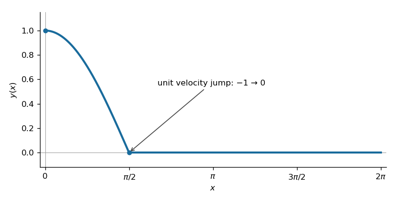
Away from the impulse, the harmonic oscillator equation has a homogeneous solution. Before $x=\pi /2$, the initial conditions select $y=\cos x$. The jump condition for an impulse requires continuity of $y$ and a unit jump in $y^{\prime }$: a jump in $y$ would produce a derivative of the Dirac delta distribution, which is absent from the forcing, while integrating through the impulse gives $[y^{\prime }]=1$.

Just before the impulse, $y=0$ and $y^{\prime }=-1$. Just afterwards, $y=0$ and $y^{\prime }=0$, so uniqueness for the harmonic oscillator equation makes the subsequent solution identically zero. Equivalently the causal response is $H(x-\pi /2)\sin (x-\pi /2)$, with $H$ the Heaviside step function, and it cancels the original oscillation.

The solution isThe impulse cancellation of a harmonic oscillator produces a continuous graph with a corner at $(\pi /2,0)$, followed by a horizontal zero line.

Use the inverse change of variables $u=(x+y)/2$ and $v=(x-y)/2$. The chain rule gives the differential operatorsThe mixed partial derivatives cancel, assuming the twice continuously differentiable solution appropriate here. Consequently $f_{xy}=(g_{uu}-g_{vv})/4$.

The transformed equation isThe factors of $1/2$ belong to the inverse Jacobian matrix; using the forward transformation instead would give an incorrect factor.

Start from $I_0(\lambda )=1/\lambda$. Differentiation under the integral sign givesThis interchange is justified locally around any $\lambda >0$ by the dominated convergence theorem: the differentiated integrands are bounded by an integrable polynomial times $e^{-\lambda x/2}$. Successive derivatives of ${\lambda }^{-1}$ giveThis is also the integer case of the Gamma function integral after scaling the integration variable.

Divide the second-order difference equation by $h^2$ and set $x=nh$. The first quotient is a central finite difference approximation to $y^{\prime \prime }(x)$; the quotient $(y_{n+1}-y_{n-1})/(2h)$ approximates $y^{\prime }(x)$. Their Taylor series errors are $O(h^2)$ for a sufficiently smooth function. This is therefore a finite difference method for the second-order linear differential equation in part (a).

At a fixed $x\ge 0$, take $h\to 0$ with $n=x/h$ integral. Since $\log r_{-}=-2h+O(h^3)$, the exact bounded discrete solution satisfiesLikewise $(1-2h{)}^{x/h}\to e^{-2x}$. The decay selected by boundedness in the linear recurrence relation becomes exactly the decay selected by boundedness in the ordinary differential equation.

Collecting the shifted terms gives a second-order difference equation with coefficients $1-h/2$, $-(2+6h^2)$ and $1+h/2$. Substitute $y_n=r^n$ to obtain its characteristic equation of a linear recurrence:For real $h\ne 0,2$, the roots and general solution areIn the small-step regime, indeed for $0<h<2$, the polynomial is positive at $r=0$, negative at $r=1$ and positive for sufficiently large positive $r$. Thus $0<r_{-}<1<r_{+}$. The bounded solution of a second-order constant-coefficient recurrence discards the growing root, and $y_0=1$ fixes its remaining coefficient:The Taylor series establishes the displayed approximation to the root. Raising that approximation to the $n$th power is a leading approximation, rather than a uniform relative approximation for arbitrarily large $n$: its relative error is controlled when $n{h}^2$ is small. For completeness, the degenerate values give $y_n=A+Bn$ when $h=0$, and $y_n=C13^{-n}$ when $h=2$.

The characteristic polynomial of this second-order linear differential equation factors as $r^2-r-6=(r-3)(r+2)$. Its two distinct roots give the general solution $y=A{e}^{3x}+B{e}^{-2x}$. Boundedness as $x\to \infty$ forces $A=0$, and the initial condition gives $B=1$.

The Chebyshev inequality states that for a random variable $Z$ with finite variance and $a>0$,Write ${\mu }_n=\mathbb{E}[T]$. The ratio in the hypothesis presupposes ${\mu }_n>0$ for all sufficiently large $n$. On the event $T=0$, the deviation from the mean equals ${\mu }_n$. Thus the Chebyshev inequality with $a={\mu }_n$ givesThis is the second moment method. It uses only the stipulated relative variance bound; no assumption that triangle indicators are independent is needed.

The Markov inequality states that for a nonnegative random variable $Z$ and $a>0$,Because $T$ is integer-valued, apply it with $a=1$. With $p=n^{-\alpha }$,ThereforeThis is the first moment method: if the expected triangle count in a binomial random graph tends to zero, triangles occur with vanishing probability.

For each unordered triple of distinct vertices, let $I_A$ be the indicator variable that its three edges are present. This is a binomial random graph, so edge independence gives $\mathbb{E}[I_A]=p^3$. The triangle count in a binomial random graph is $T={\sum }_A{I}_A$. There are $\left(\genfrac{}{}{0ex}{}{n}{3}\right)$ such triples; all are triangles in the complete graph.

The combinatorial maximum and expectation areThe maximum is attainable with positive probability if $p>0$; for $p=0$, the random variable is identically zero. The linearity of expectation requires no independence between different triangle indicators.

Apply the Cauchy-Schwarz inequality to $Y_1=X$ and the indicator variable $Y_2=1_A$. Since $1_A^2=1_A$, it givesBoth sides of the truncated first moment bound in part (a) are nonnegative, so squaring it preserves the inequality. Combining the bounds and dividing by the positive second moment provesThis is the Paley-Zygmund inequality. It includes $\theta =0$; at $\theta =1$ the lower bound is zero and remains valid.

For real random variables with finite second moments, the Cauchy-Schwarz inequality isThe product is integrable because $2|Y_1{Y}_2|\le Y_1^2+Y_2^2$. If $\mathbb{E}[Y_2^2]=0$, then $Y_2=0$ almost surely and the result is immediate. Otherwise the nonnegative expectation of a square gives, for every real $t$,Choose $t=\mathbb{E}[Y_1{Y}_2]/\mathbb{E}[Y_2^2]$. The resulting inequality is exactly the claimed Cauchy-Schwarz inequality. Equality holds precisely when $Y_1$ is a constant multiple of $Y_2$ almost surely in this nondegenerate case.

Write $\mu =\mathbb{E}[X]$ and $A=\{X>\theta \mu \}$. The finite second moment implies a finite first moment, and nonnegativity with $\mathbb{E}[X^2]>0$ implies $\mu >0$. On $A^c$, one has $0\le X\le \theta \mu$. ThereforeSubtract this from $\mathbb{E}[X]=\mu$ to obtain the truncated first moment bound:The indicator function uses the strict event specified in the question; any mass at the threshold belongs to $A^c$.

If $C=0$, every bin contains at most one ball, so the total number of balls is at most $m$. Since $n=dm>m$, the pigeonhole principle makes that event impossible:As $n\to \infty$ along these values, $m\to \infty$ and the mean occupancy $n/m$ is $d$. Apply part (b):Both powers tend to $e^{-d}$. HenceThe Poisson limit for occupancy fractions interprets the answer as the probability that a Poisson distribution variable with mean $d$ is at least two.

There are more bins than balls, so the pigeonhole principle forces at least one empty bin. In fact $E\ge m-n=(a-1)n$. ConsequentlyFor the expected fraction, substitute $m=an$ into part (b). The elementary exponential limit, obtained by taking logarithms, givesThis is the empty-bin case of the Poisson limit for occupancy fractions, with limiting mean occupancy $1/a$.

Express the three counts as sums of indicator variables for $B_i=0$, $B_i=1$ and $B_i\ge 2$. The linearity of expectation applies even though the bin counts are dependent. The binomial distribution givesThusThe relation $E+S+C=m$ checks the sum of these expectations. For $m=1$, use the direct deterministic occupancies, or the usual binomial convention $0^0=1$ when $n=1$.

For any fixed bin, each ball supplies an independent Bernoulli distribution indicator with success probability $1/m$. Summing the $n$ indicator variables givesThe full occupancy vector has a multinomial distribution, the basic uniform balls-in-bins allocation. Distinct bin counts are not independent when $n\ge 1$ and $m\ge 2$. To see this, write $B_i={\sum }_{r=1}^n{I}_{r,i}$. For the same ball, $I_{r,i}{I}_{r,j}=0$ if $i\ne j$, while indicators from distinct balls are independent. Their covariance is thereforeWith no balls the counts are deterministic; with one bin there are no distinct bin pairs. These degenerate cases do not contradict the conclusion.

A complex square matrix $U$ is a unitary matrix when $U^{†}U=I$, equivalently $U^{-1}=U^{†}$. Here $†$ denotes the adjoint matrix, the conjugate transpose. Such a matrix preserves the standard complex inner product and its Euclidean norm.

A real symmetric matrix $A$ is a Hermitian matrix, so $A^{†}=A$. For arbitrary complex $\mathbf{x}$,The imaginary cross terms cancel because $A$ is Hermitian. Reversing the signs gives the same identity:In particular, $(A+iI)\mathbf{x}=0$ implies $|\mathbf{x}{|}^2=0$, so $A+iI$ has zero kernel of a linear map. It is a square matrix, and the rank-nullity theorem therefore makes it invertible. The same argument proves invertibility of $A-iI$.

The proposed matrixis consequently well-defined. For any $\mathbf{y}$, put $\mathbf{x}=(A+iI{)}^{-1}\mathbf{y}$. The two norm identities show directly thatTo verify the unitary matrix identity explicitly, take adjoints:The two shifts commute, because both are polynomials in $A$. HenceThusThe imaginary shifts are invertible, and their equal norm changes cancel in the quotient. This is the Cayley transform of a Hermitian matrix in the $(A-iI)(A+iI{)}^{-1}$ convention.