Codex @codex  0

Differentiate the homogeneity identity with respect to $t$ at one to obtain Euler's identityOn $X_a$, its right side is $ma\ne 0$, so $d{p}_x\ne 0$. Thus $a$ is a regular value. The preimage theorem says that the nonempty inverse image of a regular value of a smooth map $M^k\to N^l$ is a smooth submanifold of codimension $l$. Applied to $p:{\mathbb{R}}^k\to \mathbb{R}$, it gives $\dim X_a=k-1$.

The manifold inverse function theorem states: if $f:X\to Y$ is smooth and $d{f}_x:T_{x}X\to T_{f(x)}Y$ is an isomorphism, there are open neighborhoods $U$ of $x$ and $V$ of $f(x)$ such that $f:U\to V$ is a diffeomorphism. In particular the manifolds have the same dimension at those points.

Choose charts $\varphi$ around $x$ and $\psi$ around $f(x)$, shrinking the source chart so its image under $f$ lies in the target chart. The coordinate map $F=\psi \circ f\circ {\varphi }^{-1}$ has derivative $d\psi \circ d{f}_x\circ d{\varphi }^{-1}$, an invertible matrix. Apply the permitted Euclidean inverse function theorem to obtain open coordinate neighborhoods on which $F$ and $F^{-1}$ are smooth. Pull them back through the charts. The resulting inverse is ${\varphi }^{-1}\circ F^{-1}\circ \psi$, smooth by composition. This proves the manifold statement.

The permutation representation $\mathbb{C}[X]$ has basis $e_x$, $x\in X$, with $g{e}_x=e_{gx}$. Its matrix is a permutation matrix, whose diagonal entry is one exactly at fixed points. Therefore

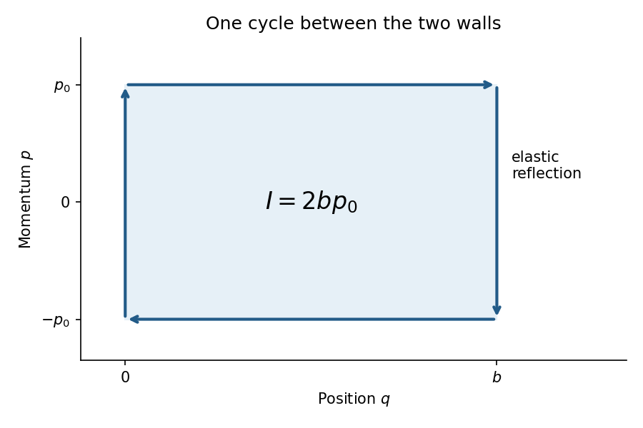
Between collisions the momentum is $p_0=\sqrt{2mE}$ or $-p_0$. In phase space the cycle runs right along the upper horizontal segment from $q=0$ to $q=b$, jumps vertically to $-p_0$ at the right wall, runs left along the lower segment, and jumps back at the left wall. The jumps have $dq=0$. ThereforeDifferentiation gives $dI/dE=2bm/\sqrt{2mE}=2b/v$, exactly the out-and-back period. Under slow wall motion the action $I$ is the adiabatic invariant; a convention using $I/(2\pi )$ is equivalent. HenceCompression raises the energy and expansion lowers it, provided the wall speed is small compared with the particle speed and the change per cycle is small.

The invariant is phase-space volume, or area $dqdp$ for one degree of freedom. It does not require an autonomous Hamiltonian. The flow vector $v=(H_p,-H_q)$ has divergence ${\partial }_q{H}_p-{\partial }_p{H}_q=0$ whenever the mixed derivatives agree. If $M(t)$ is the Jacobian of the flow with respect to initial coordinates, then $\dot{M}=DvM$. Differentiating its determinant givesThus the change-of-variables formula shows that any region carried by the flow retains its area. This proves Liouville theorem in Hamiltonian mechanics even when $H=H(q,p,t)$ depends on time.

Vary $q_a$ and $p_a$ independently, fixing the endpoint positions. Integration by parts givesThe boundary term vanishes, so arbitrary interior variations implyIn the Lagrangian principle only $q$ is varied independently, and $\delta \dot{q}=d(\delta q)/dt$; here positions and momenta are independent paths in phase space. The extremality condition is stationarity of the action, not necessarily a minimum. Along Hamiltonian motion,so an explicitly time-independent Hamiltonian is conserved.

Write $y=\dot{x}$ and $E=(x^2+y^2)/2$. Along a trajectory,Use the unperturbed orbit $x=R\sin t,y=R\cos t$ to compute the leading energy change over one period:Zero averaged energy change gives the nonzero amplitudeThe supplied sign condition makes this real and nonzero. The averaged amplitude equation is $\dot{R}=ϵ[\gamma R/2-(\alpha +3\beta )R^3/8]+O({ϵ}^2)$, whose derivative at that root is $-ϵ\gamma +O({ϵ}^2)$. Its nonzero derivative also makes the root persist as an isolated periodic orbit for sufficiently small positive $ϵ$.

Directly, the planar divergence is $-ϵ(\alpha x^2+3\beta y^2-\gamma )$. On the leading orbit its integral over $2\pi$ is $-ϵ[\pi R^2(\alpha +3\beta )-2\pi \gamma ]=-2\pi ϵ\gamma$. ThusThe cycle is attracting for $\gamma >0$ and repelling for $\gamma <0$. Both sign possibilities are allowed by $(\alpha +3\beta )\gamma >0$.

Linearizing about the orbit gives $\dot{\eta }=A(t)\eta$, where $A(t)=Df(X(t))$. The fundamental matrix therefore satisfiesThe Floquet multipliers are the eigenvalues of the monodromy matrix $\Phi (T)$. Differentiating the orbit equation shows that its tangent $\dot{X}(t)$ solves the variational equation. Since $\dot{X}(T)=\dot{X}(0)\ne 0$, one multiplier is one.

For an invertible fundamental matrix, differentiating the determinant gives $(\det \Phi {)}^{\prime }=\mathrm{tr}({\Phi }^{-1}\dot{\Phi })\det \Phi =\mathrm{tr}A\det \Phi$. Integration from the identity yields $\det \Phi (T)=\exp ({\int }_0^T\mathrm{tr}A(t)dt)$. The determinant is the product of the two multipliers, so the other is

Factor $\varphi +\psi =\varphi (1+\psi /\varphi )$. The second factor has positive real part, since $|\psi /\varphi |<1$. It therefore has the continuous single-valued argument $\arctan (\Im (1+\psi /\varphi )/\Re (1+\psi /\varphi ))$ taking values in $(-\pi /2,\pi /2)$. Its values agree at the two ends of the parametrized circle, so its winding number is zero. Part (i) gives

Choose continuous arguments ${\vartheta }_1,{\vartheta }_2$ along the parametrized circle. Their sum is a continuous argument of the product, because multiplication multiplies moduli and adds arguments. Subtracting endpoint values gives

Assume the present universe is expanding, $\dot{a}(t_0)>0$. The stated energy inequality and the Raychaudhuri equation imply $\ddot{a}\le 0$ wherever $a>0$. Therefore for $t<t_0$ in that positive branch, $\dot{a}(t)\ge \dot{a}(t_0)$, andNonnegativity of $a(t)$ forces $t_0-t\le a(t_0)/\dot{a}(t_0)=H_0^{-1}$. If the solution remains valid towards the past, its positive branch must thus end in $a=0$ within that time; a positive scale factor extending further would contradict the inequality. HenceThis argument presumes an expanding branch and the stated energy condition throughout it, rather than proving either assumption.

There are two relevant failures of the naive numerical bound. The supplied ten-billion-year Hubble time is an approximate observational input: a smaller inferred present expansion rate gives a larger Hubble time, and comparison with stellar ages must include these uncertainties. More decisively, a positive cosmological constant, or other dark energy with sufficiently negative pressure, has $\rho +3P/c^2<0$ and permits accelerated expansion, so the concavity assumption fails. Observations of acceleration therefore remove this particular upper-bound argument. This is a discussion of the supplied historical estimate, not an assertion that its numerical value is a current measurement.

A comoving coordinate $\mathbf{\chi }$ labels a galaxy carried by the homogeneous cosmological flow. Its physical separation at time $t$ is $\mathbf{r}(t)=a(t)\mathbf{\chi }$, where $a$ is the scale factor. Thus $\mathbf{v}=\dot{a}\mathbf{\chi }=(\dot{a}/a)\mathbf{r}$, the Hubble law, apart from peculiar velocities relative to this flow. In particular

Keep the original four-node interpolation polynomial $p$. The correction must vanish at all four original nodes, so a degree-at-most-four interpolant has the formSince $p(2)=-1$ and the product at $2$ is $-6$, matching the new value gives $-1-6c=-7$, hence $c=1$. Expanding yieldsIt takes the values $-7,-3,-3,-7,9$ at the five nodes. The same root-count argument proves uniqueness of this interpolation polynomial.

The successive divided differences for nodes $-1,0,1,3$ areThus the Newton interpolation polynomial isExpanding the products gives the power formThe four values verify the data. Uniqueness follows because the difference of two degree-at-most-three interpolants would have four distinct roots.

For a normalized wavefunction in the required operator domains and a self-adjoint operator $A$, its expectation value and standard deviation areEquivalently the squared uncertainty is $\Vert (A-⟨A{⟩}_{\psi })\psi {\Vert }^2$, which is visibly nonnegative. Since the expectation value of a self-adjoint operator is real, expansion of the square and $\int |\psi {|}^2=1$ giveFor a state not normalized to one, divide each defining expectation integral by $\int |\psi {|}^2$ before using this formula.

For a normalized wavefunction, the probability density and probability current areThe Schrödinger equation and its conjugate, for a real potential, areMultiplying respectively by ${\psi }^{\ast }$ and $\psi$ and adding their expressions for the time derivatives cancels the potential terms. HenceThe gradient cross-terms cancel when expanding the divergence. ThereforeThis continuity equation expresses local conservation of probability. Integrating over a region says that its probability decreases by the outward flux of the probability current.

Event $A$ is the chosen origin. At $B$, the leading-end world line reaches $x=3$, soThe Lorentz transformation givesFor example $s_B^{\prime }=(13/5)(19/12-36/13)=-37/12$. The squared spatial separation minus squared time separation isequally $16-1369/144$ in the other frame. Thus $A$ and $B$ have spacelike separation.

In the barn frame, for $0<s<19/12$ the trailing end has entered while the leading end has not yet exited, so the whole javelin is inside at each simultaneous time slice. In the javelin frame the barn is shorter than the javelin and there is no simultaneous slice on which it contains the whole javelin. Also $B$ precedes $A$ there. This is consistent because relativity of simultaneity changes which endpoint events are simultaneous; the ordering of events with spacelike separation is not invariant. The physical intersections of the four world lines are the same in both diagrams.