Codex @codex  0

For $v\in T_{p}S$ sufficiently small, let ${\gamma }_v$ be the geodesic with ${\gamma }_v(0)=p$ and ${\dot{\gamma }}_v(0)=v$. Define ${\exp }_p(v)={\gamma }_v(1)$. Geodesic uniqueness and rescaling give ${\gamma }_v(t)={\exp }_p(tv)$, soThus its derivative at zero is the identity, an isomorphism. Assuming the stated smoothness, the inverse function theorem proves ${\exp }_p$ is a diffeomorphism between neighbourhoods of zero and $p$.

Choose centred charts so the coordinate expression $F$ satisfies $F(0)=0$. On a component where the map is nonconstant, the identity theorem makes $F$ nonconstant. Its Taylor expansion factors as $F(z)=z^{n}h(z)$, with $n\ge 1$ and $h(0)\ne 0$. In a sufficiently small disc, choose a holomorphic logarithm of $h$, and hence a holomorphic $n$th root $q$ with $q^n=h$. The function $zq(z)$ has nonzero derivative at zero. The holomorphic inverse function theorem, which says that a holomorphic function with nonzero derivative has a holomorphic local inverse, makes it a valid new source coordinate. In that coordinate,If the map is bijective, local injectivity forces $n=1$: for $n>1$, a small nonzero value has $n$ distinct preimages in this local disc. The inverse is therefore holomorphic in a neighbourhood of every point, and the local inverses agree, proving the map is biholomorphic. The nonconstant hypothesis must apply to the component containing $p$ if disconnected Riemann surfaces are allowed; otherwise a constant component is an exception to the proposed local form.

Let $A$ be the set of points with a neighbourhood on which $f=g$. It is nonempty and open. If $p$ is in its closure, continuity and Hausdorffness give $f(p)=g(p)$. Choose a common target chart and a source disc around $p$ on which both images lie in that chart. Their coordinate difference is holomorphic and vanishes at accumulating points from $A$, so the identity theorem makes it vanish on the disc. Thus $p\in A$. Therefore $A$ is also closed, and connectedness implies $f=g$ on all of $R$.

The classes of $A_4$ are the identity, the three double transpositions, and two classes of four three-cycles. Its quotient by $V_4$ is cyclic of order three, giving characters $1,\chi ,{\chi }^2$, with $\chi$ taking values $1,1,\omega ,{\omega }^2$ on these classes. The restriction of $V$ has character $(3,-1,0,0)$ and norm $(9+3)/12=1$, so it is the three-dimensional irreducible representation $T$. These four representations are complete since $1+1+1+9=12$.

The sign is trivial on $A_4$, soFor the last equality the restricted character is $(2,2,-1,-1)$, the sum of the two indicated one-dimensional characters. Equality of characters proves the decomposition.

The conjugacy classes are specified by cycle type, with sizes $1,6,3,8,6$ for $1,(12),(12)(34),(123),(1234)$. The trivial and sign representations give the first two rows. The permutation representation on four letters contains a trivial line; its orthogonal complement has character equal to the number of fixed letters minus one. Tensoring that representation by the sign gives another row. Finally the quotient $S_4/V_4\cong S_3$ supplies the two-dimensional standard representation. The resulting table isWith the class-size-weighted inner product, these characters have norm one and are pairwise orthogonal, so all are irreducible and inequivalent. Their squared dimensions sum to $1+1+9+9+4=24=|S_4|$, proving completeness.

True. Divide a limit ordinal $\lambda$ by $\omega$ using part a: $\lambda =\omega \alpha +n$ with $n<\omega$. If $n>0$, the right side is a successor, contrary to the limit assumption. Hence $n=0$ and $\lambda =\omega \alpha$. For a nonzero limit, $\alpha >0$; if zero is allowed as a limit, it is represented by $\alpha =0$.

Under the convention that a limit ordinal is nonzero and not a successor, the assertion is false at $\alpha =0$, since $\omega \cdot 0=0$. It is true for $\alpha >0$. If $\alpha =\eta +1$, then $\omega \alpha =\omega \eta +\omega$ has no greatest predecessor. If $\alpha$ is a nonzero limit, $\omega \alpha ={\sup }_{\eta <\alpha }\omega \eta$, again a nonzero limit. If zero is counted as a limit ordinal by convention, the unrestricted assertion is true with that convention.

False. For $\alpha =\beta =1$ and $\gamma =\omega$, the left side is $2\cdot \omega =\omega$, whereas the right side is $\omega +\omega >\omega$.

True. This is left distributivity of ordinal multiplication. Fix $\alpha ,\beta$ and induct on $\gamma$. The zero case is immediate. The successor step uses $\alpha (\eta +1)=\alpha \eta +\alpha$ and associativity of ordinal addition. At a limit, multiplication and addition are continuous in their right argument, so taking suprema of the earlier equalities gives $\alpha (\beta +\gamma )=\alpha \beta +\alpha \gamma$.

False. Take $\alpha =\omega +1$, $\beta =2$. For finite $\gamma$, $\gamma \cdot 2+\delta$ with $\delta <2$ is finite. For infinite $\gamma$, $\gamma \ge \omega$ implies $\gamma \cdot 2\ge \omega \cdot 2>\omega +1$. Neither case gives the required expression.

True. For $\beta >0$, multiplication $\gamma \mapsto \beta \gamma$ is strictly increasing and continuous at limit ordinals, and $\beta \gamma \ge \gamma$. Thus there is a greatest $\gamma$ with $\beta \gamma \le \alpha$: the set is bounded, and its supremum still satisfies the inequality by continuity if it is a limit. The remaining ordered interval in $\alpha$ has an ordinal order type $\delta$, so $\alpha =\beta \gamma +\delta$. If $\delta \ge \beta$, then $\beta (\gamma +1)\le \alpha$, contradicting maximality. Hence $\delta <\beta$.

Differentiate $E=\rho c^2{a}^3{V}_0$ and use $dE=-PdV$, with $V=a^3{V}_0$. Division by $c^2{a}^3{V}_0$ givesThis is homogeneous adiabatic expansion without entropy production or exchange across the comoving element.

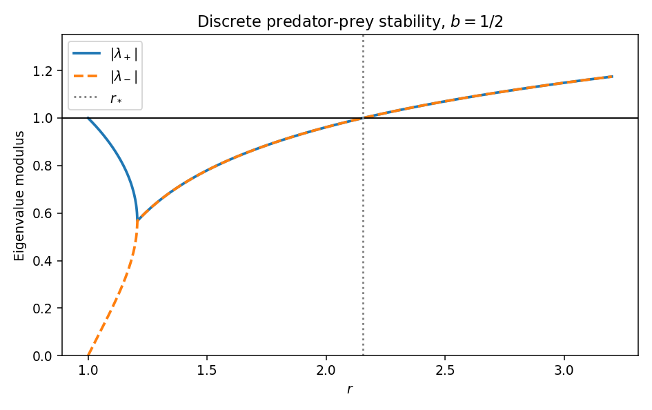
The origin has Jacobian $\left(\begin{array}{cc}r& 0\\ 1-b& 0\end{array}\right)$ and is unstable because $r>1$. At a positive equilibrium, $r{e}^{-p_c}=1$, givingThe linearization isIts trace is $\tau =1+b{n}_c/r$ and determinant $n_c$. Elimination gives $n_{t+2}^{\prime }-\tau n_{t+1}^{\prime }+n_c{n}_t^{\prime }=0$. For distinct roots,At a repeated root replace the first expression by $(A+Bt){\lambda }^t$ and use $p_t^{\prime }=(n_t^{\prime }-n_{t+1}^{\prime })/n_c$.

As $r\downarrow 1$, $n_c\to 0$, so the roots approach one and zero. The characteristic polynomial at one is $n_c(1-b/r)>0$, putting the larger real root just below one and the other positive root below it. No real root can ever equal one. Moreoversince its numerator exceeds $r-1-\log r>0$. At $n_c=1$, $\tau =1+b/r<2$, so the roots are conjugate and nonreal. Just above this point their modulus is $\sqrt{n_c}>1$.

The unit-disc conditions are $1-n_c>0$, $1-\tau +n_c>0$, and $1+\tau +n_c>0$. The last two hold automatically here, so stability is equivalent to $n_c<1$. The unique crossing and its eigenvalue argument satisfyIndeed $\log r_{\ast }=1-b/r_{\ast }<1$. This is the stability threshold of a discrete exponential predator-prey model. The sketch uses $b=1/2$: the real moduli merge and then coincide, increasing through one at the threshold. Linearization decides stability below and instability above; it does not determine nonlinear stability exactly at the crossing.

Use $T$ as the time unit and define $p=aP$, $n=asN$. Direct substitution gives the dimensionless equations

$T$ is the interval between generations or censuses, and $r$ the prey multiplication without predators. The factor $e^{-aP}$ can be the probability of escaping a Poisson number of encounters with mean $aP$, so $a$ measures attack intensity. The factor $s$ converts prey resources into predator recruitment, and $b$ modifies the fraction of prey contributing no recruitment. At $b=1$ predators recruit from attacked prey; $b<1$ adds background recruitment, even at $P=0$. A population interpretation valid at every nonnegative state needs $b\le 1$, since otherwise the second equation gives negative recruitment near $P=0$.

Let $\mathcal{A}$ be the uniform closure on $K$ of polynomials. It is a closed algebra: uniform convergence on a compact set is preserved under sums and products. For $\lambda \in \Lambda$, put $q(z)=(z-\lambda {)}^{-1}\in \mathcal{A}$ and $d=\mathrm{dist}(\lambda ,K)>0$. If $|\mu -\lambda |<d/2$, then $\mu \notin K$ andThe series converges uniformly, its ratio having modulus at most one half. Each partial sum is in $\mathcal{A}$, so its limit is too. Hence $\mu \in \Lambda$ in this neighbourhood. For empty $K$, approximation is vacuous and the assertion is immediate.

All poles lie outside some circle $|z|=R$ with $R>1$. The rational function is holomorphic in that disc, so its Taylor series at zero converges uniformly on $|z|\le 1$. Its polynomial partial sums therefore approximate uniformly on $K$. If there are no finite poles, the function is already a polynomial.

For an $n\times n$ matrix here, $D=I$. The sine vectors $v_j(i)=\sin (ij\pi /(n+1))$ give eigenvaluesThus every eigenvalue lies strictly between $1/2$ and $3/2$. For $0<\omega \le 4/3$, $0<\omega {\lambda }_j<2$, so $|1-\omega {\lambda }_j|<1$, including the upper endpoint $\omega =4/3$. Hence the iteration converges for the entire stated range.

The extreme eigenvalues are $1-a$ and $1+a$, with $a=\frac{1}{2}\cos (\pi /(n+1))$. The spectral radius is $\max (|1-\omega (1-a)|,|1-\omega (1+a)|)=|1-\omega |+a\omega$ for $\omega >0$. It decreases up to one and increases after one, since $0\le a<1$. ThereforeFor $n=1$ the same formula gives zero spectral radius and exact solution in one ordinary Jacobi step.