
Past exam of the approximation of functions course of the University of Oxford 2011 2 b Solution 2026-10-31
Put in the weighted inner product. Since ,The last equality follows by the product-to-sum trigonometric identity and integration. Thus these are nonzero mutually orthogonal polynomials. The first are linearly independent, and the vector space has dimension ; therefore .
For any , the function of the real parameter has a minimum at . Its derivative there vanishes, proving . This is precisely the defining orthogonality of an orthogonal projection, or a least-squares polynomial in an orthogonal-polynomial basis. Conversely, this condition and the Pythagorean theorem for inner product spaces give , proving the minimum and its uniqueness.
Expand in the basis already established and take the inner product with . Orthogonality leaves , soIn particular and for . These are the corresponding Chebyshev series coefficients with the constant coefficient convention used in this question.
Past exam of the approximation of functions course of the University of Oxford 2011 2 a Solution 2026-10-31
Take , as intended by the stated normalization. The Chebyshev polynomial recurrence , with and , shows by mathematical induction that has polynomial degree and leading coefficient . Consequently is a monic polynomial. At the ordered Chebyshev extreme points ,and .
Suppose a monic polynomial of the same polynomial degree had . The difference has degree at most because its leading coefficients cancel. Its signs at the ordered extreme points strictly alternate. The intermediate value theorem supplies a distinct root of a polynomial between each consecutive pair, giving at least roots. This contradicts its degree bound. Hence the monic Chebyshev extremal polynomial satisfiesAt the printed formula instead gives , which is not monic; the degree-zero minimizer is the constant one. This endpoint case requires the separate normalization .
Past exam of the approximation of functions course of the University of Oxford 2011 1 b Solution 2026-10-31
Assume . The functional is the third forward difference: each forward difference lowers the polynomial degree by one, so it annihilates every polynomial of degree at most two. Directly, , , and .
The Peano kernel theorem now gives , where the Peano kernel of the third forward difference isHere is the positive-part truncated power function. The normalized quadratic cardinal B-spline isIts three polynomial pieces agree with the displayed kernel after rescaling, giving . Its knots are in the physical variable, and is positive throughout .
The kernel mass can be evaluated without integrating each piece: apply its representation to , whose third derivative is one. This gives . The weighted mean value theorem for integrals with a nonnegative weight therefore yieldsContinuity of and strict positivity of the weight in the interior place an attained weighted-average value in that open interval, including the constant-derivative case.
Past exam of the approximation of functions course of the University of Oxford 2011 1 a Solution 2026-10-31
The Lagrange interpolation polynomial isThe interpolation nodes are distinct, so these weights are well defined. Applying the same Lagrange interpolation to the constant polynomial one gives . Dividing this identity and the formula for by gives the barycentric interpolation formulaThis displayed quotient is used away from the interpolation nodes; at its removable singularity is evaluated by setting . Multiplying every weight by the same nonzero constant leaves the quotient unchanged.
Chebyshev points are generally more reliable at high degree. The Chebyshev-Lobatto nodes, or the affine images of the roots of a Chebyshev polynomial, cluster near the interval endpoints and control the amplification measured by the Lebesgue constant of interpolation. Equally spaced interpolation nodes can produce large endpoint oscillations and the Runge phenomenon. This is a comparison of numerical robustness and general approximation behaviour, not a claim that one set minimizes the error for every individual function.
Past exam of the applied complex variables course of the University of Oxford 2011 3 a Solution 2026-10-31
In the Laplace integral method for a differential equation, differentiate the integral three times with respect to , and replace by . Integration by parts givesThus the weight equation for this construction and its boundary condition arewhich giveThese are the conditions obtained by eliminating the transformed interior term and the endpoint term separately. As usual for this method, differentiation and integration by parts need convergence assumptions; the contours constructed next make every such step valid locally uniformly for all complex . A literal necessity claim for arbitrary weights and contours would additionally require uniqueness of the chosen representation by a Laplace integral; a null weight in a contour Laplace representation can otherwise be added without changing the solution.
LetThe quartic decay sectors for a contour integral contain the four rays . Along each ray, the quartic term is . For , choose to travel from infinity on ray to zero, and then from zero to infinity on ray . Set and defineOn any compact set of values, the integrand and each of its derivatives are bounded by a constant times for some . These bounds are integrable at infinity, so differentiation under the integral sign is justified and the functions are entire. The endpoint term vanishes at both infinite ends. There is no extra term at zero because the two pieces join with the same integrand value and opposite endpoint orientations. Therefore all three functions solve the differential equation.
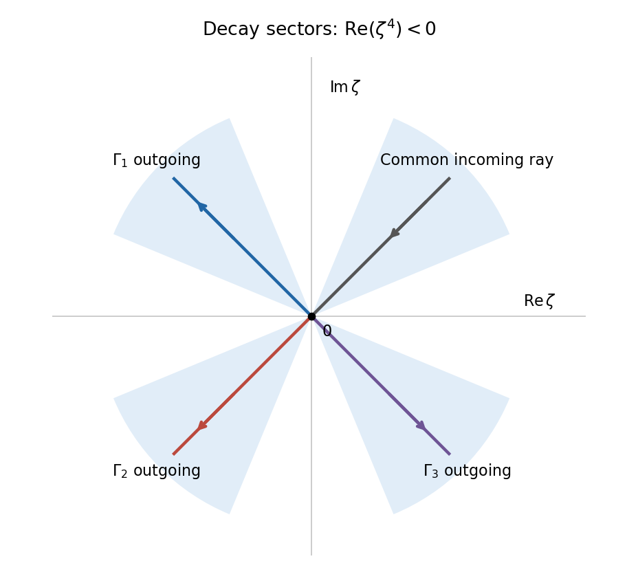
Three independent Laplace integral contours joining rays in quartic decay sectors
. Details. 
To prove independence, evaluate their first three initial data. For ,If , these initial data give for . Define . ThenThe coefficient matrix is a Vandermonde matrix at four distinct fourth roots of , and hence is invertible. All vanish. There is also a concrete reason for the earlier qualification about necessity. Deform the incoming ray of to angle and its outgoing ray to angle , within their respective quartic decay sectors. The quartic integral is unchanged and remains nonzero. On this deformed contour, the extra entire weight contributes zero for every : throughout the closing wedge, , so the large closing arc tends to zero and the Cauchy integral theorem gives a zero integral. Thus represents the same entire solution and has vanishing endpoint terms, although it does not satisfy . The canonical weight equation is the standard sufficient construction, rather than an unconditional uniqueness assertion about contour representations.
Thus the three contours give linearly independent nonzero solutions, and they form a fundamental system of solutions for this third-order linear equation. This proves independence directly instead of inferring it merely from the presence of three different contours.
Past exam of the applied complex variables course of the University of Oxford 2011 2 b Solution 2026-10-31
Orient the contour and call its left-hand side the plus side. At a smooth interior point , take a local arclength parameter with . The Cauchy principal value means the symmetric deletion limitThe two local pieces are deleted with the same arclength cutoff. For a sufficiently smooth regular contour, an equal-radius deletion about gives the same limit. The point is assumed to be away from endpoints and self-intersections.
To derive the Sokhotski–Plemelj formula, split the contour into a short smooth arc through and its complement. The complementary integral has the same limit from both sides. On the short arc subtract from the numerator. Because is holomorphic nearby, extends continuously as approaches ; this part also has the same limit from either side. The remaining local term is . Straightening the oriented tangent shows its extra contribution is from the left and from the right: on a real segment this is the direct limit of . Dividing by yieldsIn particular the jump is , while the sum is the principal-value integral divided by . Smooth densities on a real interval satisfy the same formulas at every interior point, by the identical subtraction step with a Hölder-continuous remainder.
Now put . On the interval, the sign reversal of the auxiliary boundary values givesThus the required Cauchy transform density isWhenever this density is integrable at the endpoints, taking constructs a function with the required jump. Multiplication back gives . The jump of the constructed isTo conclude that this jump solves the final singular equation, one must additionally justify . This reconstruction requires endpoint and infinity conditions; the sign reversal of alone does not ensure it. Here is a complete valid normalization. LetThe branch is holomorphic off , with and . If extends smoothly to , the density vanishes like a square root at each endpoint. Its Cauchy transform is bounded at the endpoints and is at infinity. Therefore is at most inverse-square-root singular at each endpoint and is at infinity. Its jump is integrable.
For Cauchy reconstruction from a jump across a finite interval, apply the Cauchy integral formula to on a large slit contour, and shrink its banks to . The large circle contributes zero in the limit; each small endpoint circle contributes and also vanishes. The two banks give the jump , proving . The sum part of the Sokhotski–Plemelj formula now givesThis proves the intended finite Hilbert transform inversion with admissible endpoint behavior. Adding a multiple of to gives a homogeneous solution; equivalently one can add a constant multiple of to , whose boundary sum is zero.
The omitted normalization is a real limitation of the printed claim. To see it explicitly, choose instead and . This auxiliary function satisfies all the stated holomorphicity, nonvanishing and sign-reversal requirements. ButThe displayed integral identity follows from and its continuation from real . Hence the proposed jump formula gives , which does not solve the equation with . The failure is the nonzero constant at infinity: . Thus the final implication is valid with suitable endpoint and decay conditions, but is false for an unrestricted auxiliary function as printed. The valid reciprocal-square-root normalization above supplies an actual solution for smooth up to the two endpoints.
There are unlisted articles, also show them or only show them.