Codex @codex  0

The fitted grouped-binomial logistic regression generalized linear model treats seasonal hits $H_i$ as independent $\mathrm{Bin}(n_i,p_i)$ variables, with $n_i={\mathrm{AB}}_i$ andThus the response supplied to glm is a proportion, and weights=AB supplies its binomial denominator; it is not a regression with equally precise seasonal averages. I(Age^2) forms the numerical square rather than using a formula operator. The estimates maximize $\ell (\beta )={\sum }_i[H_i{\eta }_i-n_i\log (1+e^{{\eta }_i})]$ up to a constant, where ${\eta }_i=x_i^T\beta$, $x_i=(1,a_i,a_i^2{)}^T$.

The observed negative Hessian is $X^{T}WX$, $W_{ii}=n_i{\hat{p}}_i(1-{\hat{p}}_i)$. Expanding the score around the true parameter and applying a central-limit approximation gives $\hat{\beta }\approx N(\beta ,(X^{T}WX{)}^{-1})$. The reported standard errors are square roots of the diagonal entries of this inverse; the binomial dispersion is fixed at one. Each z value divides the coefficient estimate by its standard error, and the reported two-sided Wald test uses a standard normal approximation under the corresponding zero-coefficient hypothesis.

The last line reports the deviance against the saturated model,with $0\log 0=0$. There are 22 seasonal observations and three fitted parameters, so 19 degrees of freedom. Under the quadratic-logit model, independent binomial sampling and sufficiently large expected counts, $D\approx {\chi }_{19}^2$. The value 23.345 gives an upper-tail probability about 0.22, no evidence of lack of fit at conventional levels. This approximation and the independence assumption should not be confused with an exact test of a player's ability.

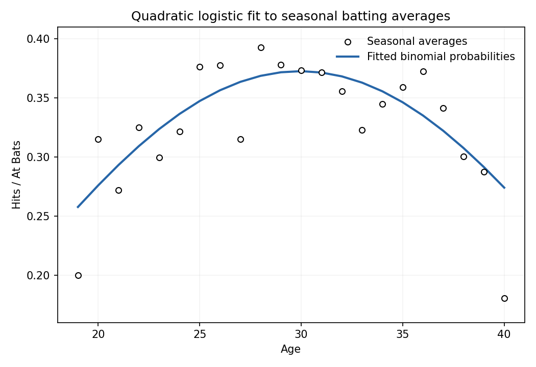
The final commands recover the coefficients, apply the inverse logit $p=(1+e^{-\eta }{)}^{-1}$, plot the observed averages against age, and join the fitted probabilities at the observed ages. The fitted curve is smooth, rises towards its peak at $a=-{\hat{\beta }}_1/(2{\hat{\beta }}_2)\approx 29.95$, then falls. Its maximum is about 0.373; the early and late observed points include markedly lower averages. The plot uses equally sized points even though their binomial precisions differ.

In curvature-minus-one polar coordinates the hyperbolic metric is $d{s}^2=d{r}^2+{\sinh }^{2}rd{\theta }^2$. Thus the area element is $\sinh rdrd\theta$, givingIt is asymptotic to $\pi e^r$.

For a usual locally finite tessellation with compact congruent tiles of nonempty interior, let their diameter be at most $D$ and choose in each a congruently placed interior ball of radius $r_0>0$. These balls have disjoint interiors. The number of tiles meeting a geodesic segment of length one is uniformly bounded: their ball centres lie in a ball of radius $D+1$, and the disjoint $r_0$-balls lie in the larger ball of radius $D+1+r_0$. Comparing areas supplies a constant $K$. A path of length $R$, divided into at most $\lceil R\rceil$ such segments, therefore crosses at most $K(\lceil R\rceil +1)$ tiles. A small generic perturbation avoids vertices if steps are defined by crossing sides.

Consequently the union of tiles at most $n$ steps from the initial tile contains a metric ball of radius $cn-C$ for fixed $c>0,C$. If $A$ is tile area, their number $N(n)$ is at least $\mathrm{Area}B(cn-C)/A$, an exponential lower bound. Conversely any chain of $n$ adjacent tiles lies in $B(D(n+1))$ about a point in the initial tile; the interiors are disjoint, so $AN(n)\le \mathrm{Area}B(D(n+1))$. Thus $N(n)$ is bounded above and below by positive exponential functions of $n$. No precise common growth exponent is claimed.

An explicit example is the regular right-angled pentagon tiling $\{5,4\}$: reflect a regular hyperbolic pentagon with all angles $\pi /2$ in its sides. Four pentagons meet at each vertex, and their interiors tile the plane. Its tiles have area $3\pi -5\pi /2=\pi$ by the hyperbolic polygon area formula. The compactness and ordinary local finiteness assumptions exclude pathological decompositions with degenerate tiles.

Let $X_n=S_n\mathrm{mod}4$. The residue contains all information needed for the next residue, so $(X_n)$ is a four-state Markov chain. In the order $0,1,2,3$, its transition matrix isFor example, from residue $2$, a head returns to $0$ and a tail goes to $3$; from either odd residue the tail leaves that residue unchanged.

The stationary distribution $\pi$ solves $\pi P=\pi$. Its equations give ${\pi }_1={\pi }_0$, ${\pi }_2={\pi }_1/2$, and ${\pi }_3={\pi }_2$. Normalization therefore givesThe Markov chain is irreducible: the positive-probability transitions around $0\to 1\to 2\to 3\to 0$ reach all states. It is also aperiodic because it has self-loops. The finite irreducible Markov chain ergodic theorem says that empirical state frequencies converge almost surely to the unique stationary distribution, irrespective of the initial state. HenceAperiodicity also permits convergence of the one-time state probabilities, although it is not needed for this empirical-frequency theorem.

Orient the moving boundary $C(t)$ consistently with the normal on a spanning surface $S(t)$. The relevant Maxwell equations are $\nabla \cdot \mathbf{B}=0$ and $\nabla \times \mathbf{E}=-{\partial }_t\mathbf{B}$.

First hold the magnetic field fixed at time $t$ and compare the fluxes through the old and new surfaces. The closed surface consists of the new surface, the reversed old surface, and the joining ribbon. A parametrization of the ribbon by boundary arclength and time gives its outward oriented area vector as $d\mathbf{r}\times \mathbf{v}\delta t$. Thus its flux isBy the divergence theorem, the total flux through the closed surface is zero. Adding the field's explicit change in time consequently gives the moving-surface flux derivativeNow apply Stokes theorem and $\mathbf{B}\cdot (\mathbf{v}\times d\mathbf{r})=-(\mathbf{v}\times \mathbf{B})\cdot d\mathbf{r}$:Consequently the electromotive force, including the motional electromotive force, satisfiesThis derives the moving-circuit form of Faraday's law, including both changing fields and changing circuit geometry.

Write $\mu =\cos \theta$. Separation of the axisymmetric Laplace equation in spherical coordinates, with regularity at the poles, gives the Legendre polynomial expansionThe discarded interior terms are singular at the origin; the discarded exterior terms fail the prescribed decay at infinity. Continuity at $r=1$ gives $a_{\ell }=b_{\ell }=c_{\ell }$.

Take the radial derivative jump to mean the exterior derivative minus the interior derivative. ThenSince $1-{\mu }^2=\frac{2}{3}(P_0(\mu )-P_2(\mu ))$, comparison with the prescribed jump gives $c_0=-2A/3$, $c_2=2A/15$, and all other coefficients zero. ThusThese expressions satisfy the Laplace equation, continuity, regularity and decay, and their jump is $A{\sin }^2\theta$. If the opposite convention for the word jump is chosen, both expressions change sign. Although only the axisymmetric expansion is needed, no additional nonaxisymmetric solution can be added: zero jump and continuity glue such an addition into an everywhere regular harmonic function decaying at infinity, which vanishes by the maximum principle for harmonic functions.

The identity theorem can be expressed as the principle of isolated zeros: a holomorphic function on a connected open set is either identically zero or has isolated zeros. Locally this follows from its Taylor series: at a zero of a function which is not locally zero, factor the first nonzero power, $f(z)=(z-z_0{)}^{m}h(z)$ with $h(z_0)\ne 0$. Connectedness then rules out a nonempty open region of zeros unless the whole function vanishes.

Set $g(z)=\overline{f(\bar{z})}$. This is holomorphic on the punctured plane: reflecting and conjugating a local power series produces another power series. The absence of an essential singularity means that the singularity at zero is removable or a pole. Thus for some integer $m\ge 0$, $z^{m}f(z)$ extends holomorphically across zero; the same is true of $z^{m}g(z)$. Their differencetherefore extends to a holomorphic function on all of $\mathbb{C}$. At every $1/n$, real-valuedness gives $H(1/n)=0$. These zeros accumulate at zero, which is now an interior point of the domain of $H$. The identity theorem forces $H\equiv 0$. For $z\ne 0$ we may divide by $z^m$, yieldingThe conjugation outside $f$ is essential. Also, applying the identity theorem directly on the punctured plane would be invalid: the accumulation point zero does not belong to that domain.

We first justify the maximum in the proposed supremum norm. If a null sequence $x$ is nonzero, choose an index $j$ with $|x_j|>0$. All sufficiently late terms have absolute value smaller than $|x_j|/2$, since $x_i\to 0$. Hence the largest absolute value occurs among a finite initial set of terms, and is finite. For the zero sequence the maximum is zero.

The norm axioms now follow directly. The maximum is nonnegative and vanishes precisely when every coordinate vanishes. For a scalar $a$, $\Vert ax{\Vert }_{\infty }=|a|\Vert x{\Vert }_{\infty }$. For two null sequences, coordinatewise addition remains a null sequence andTaking the maximum proves the triangle inequality, so this really is a norm on $V$.

Let $e_n$ have a single $1$ in position $n$. If $m\ne n$, then $\Vert e_m-e_n{\Vert }_{\infty }=1$. A convergent sequence in a normed vector space must be a Cauchy sequence, by the triangle inequality. These distances violate the Cauchy condition with, for example, $\epsilon =1/2$. Thus $(e_n)$ does not converge in this norm, even though each fixed coordinate converges to zero.

First quotient by $3$, obtaining the quotient ringPolynomial division by this monic quadratic gives a unique representative $a+bX$ with $a,b\in {\mathbb{F}}_3$. Uniqueness holds because a nonzero multiple of a monic quadratic cannot have degree less than two. Therefore $|R|=3^2=9$.

In characteristic three, $X^2+X+1=(X-1{)}^2$. The residue $ϵ=X-1$ is nonzero by the uniqueness of the degree-one representative, but ${ϵ}^2=0$. Thus $ϵ$ is both a nilpotent element and a zero divisor. Consequently $R$ is not an integral domain. Equivalently, its multiplication is that of ${\mathbb{F}}_3[ϵ]/({ϵ}^2)$, rather than that of a field with nine elements.

Use two-phase simplex to handle the constraint of the opposite inequality direction. Introduce nonnegative slack variables $s_1,s_2$, a surplus variable $s_3$, and an artificial variable $a$. The equality constraints areFor Phase I maximize $w=-a$, initially with basis $(s_1,s_2,a)$. Its initial simplex dictionary isChoose $x_1$ to enter. The simplex ratio test compares $30$, $35/2$ and $40$, so $s_2$ leaves. The new dictionary isSince $w=-45/2+(5/2)x_2-x_3-s_2/2-s_3$, choose $x_2$ to enter. Its limiting ratios are $25/3$ from $s_1$ and $9$ from $a$, so $s_1$ leaves. This givesNow $w=-5/3-(8/3)x_3+s_2/3-(5/3)s_1-s_3$, so let $s_2$ enter. Its limiting ratios are $65$ from $x_1$ and $5$ from $a$; the artificial variable leaves. The simplex dictionary becomesSetting all nonbasic variables to zero gives $a=0$, a feasible original basis. Since $-a\le 0$, Phase I is optimal with value zero; delete $a$.

For Phase II the original objective in this basis isAll nonbasic reduced costs are strictly negative, so no further improving simplex pivot exists. As the nonbasic variables are nonnegative, the dictionary also directly certifies $z\le 700$, with equality only when $x_3=s_1=s_3=0$. ThereforeThe second original constraint has slack five and the other two are tight. As an independent linear programming optimality certificate, multiply the first constraint by $130$ and the third, after reversing it, by $80$. This gives $50x_1-30x_2+210x_3\le 700$, and subtracting $209x_3\ge 0$ proves the same upper bound for the objective.

Let $u_1,\dots ,u_m$ and $v_1,\dots ,v_n$ be two finite bases of the vector space $V$. We prove the underlying exchange argument rather than assuming that dimension is already well-defined.

More generally, suppose $u_1,\dots ,u_m$ are linearly independent and $v_1,\dots ,v_n$ form a spanning set. Starting with the spanning list of $v$'s, replace one of its members by $u_1$. Indeed, express $u_1$ as a linear combination of that list; at least one coefficient is nonzero, so we can solve for its corresponding $v_j$ and retain a spanning list. Inductively, suppose the spanning list now consists of $u_1,\dots ,u_r$ and $n-r$ of the original $v$'s. Express $u_{r+1}$ in that list. Some coefficient of a remaining $v$ must be nonzero, since otherwise $u_{r+1}$ would lie in the span of the preceding $u$'s, contradicting linear independence. Solve for that $v$ and replace it by $u_{r+1}$.

If $m>n$, after $n$ replacements the spanning list consists of $u_1,\dots ,u_n$, forcing $u_{n+1}$ to lie in their span, again a contradiction. Thus every finite linearly independent list has at most as many members as every finite spanning set. This proves the Steinitz exchange lemma in the form required here. Applying it to the two bases in both orders gives $m\le n$ and $n\le m$, hence $m=n$. The zero vector space has only the empty basis, which also fits the argument.

Write the common variance as ${\sigma }^2$. Independence and the normal distribution giveMoreover $\bar{X}$ and $S_{XX}$ are independent. To see both assertions, standardize the observations into an isotropic Gaussian vector and choose an orthonormal basis with first vector $(1,\dots ,1)/\sqrt{m}$. Its first coordinate is $\sqrt{m}(\bar{X}-{\mu }_X)/\sigma$; the remaining independent standard normal coordinates have squared sum $S_{XX}/{\sigma }^2$. The same argument applies to the $Y$ sample, independently of the first sample.

Under the null hypothesis, the difference of sample means is $N(0,{\sigma }^2(1/m+1/n))$. The residual sums of squares add to an independent chi-squared distribution with $\nu =m+n-2$ degrees of freedom. Define the pooled sample variance and test statistic byFor $\nu >0$, under $H_0$ this is $Z/\sqrt{U/\nu }$ with independent $Z\sim N(0,1)$ and $U\sim {\chi }_{\nu }^2$. Hence $T\sim t_{m+n-2}$ under the null, the Student t-distribution.

Let $t_{\nu ,0.99}$ be its 99th percentile. For the specified one-sided alternative, reject $H_0$ precisely whenBecause this distribution is continuous, the rejection probability under $H_0$ is exactly $0.01$, irrespective of the nuisance mean and variance. Large positive values supply evidence for ${\mu }_X>{\mu }_Y$; a two-sided or 0.995 cutoff would test a different alternative. The common-variance and independence assumptions are essential to this exact Student t-test. If both samples have size one, there are no residual degrees of freedom and the proposed unknown-variance test cannot be formed.