
The Steinitz exchange lemma states that if are linearly independent and span a vector space , then and some of the can be replaced by while preserving the spanning set property.
Here is the exchange argument. Suppose that after replacements, a spanning set iswhere the remaining have been relabelled if necessary. Express as a linear combination of this family. At least one remaining has a nonzero coefficient; otherwise belongs to the span of , contradicting linear independence. Relabel this entry . Solving for shows that it lies in the span ofThe new family therefore still spans . Starting at repeats this step until all independent vectors have been inserted. If , after steps the next would lie in the span of , a contradiction. Thus , and the construction proves the replacement assertion as well.
The vectors are linearly independent ifThey span if every is a linear combination with real coefficients. They form a basis of if they are linearly independent and span . Equivalently, every has exactly one such representation: existence is the spanning set condition, and subtracting two representations shows that uniqueness is precisely linear independence.
For the thin spherical charge layer limit, smoothness of givesThus the shell's total electric charge tends to while its thickness tends to zero. At each fixed , the observation point eventually lies outside the shell, whereas at each fixed the interior electric field is unchanged. The limiting electric field away from the sphere is thereforeIts outward-minus-inward jump isPhysically, the limit is a uniformly charged ball of charge density , together with an infinitesimally thin spherical shell of uniform surface charge densityIndeed its electric charge is , and the standard normal electric field jump is . The surface charge density can have either sign, or vanish, according to .
The order of limits matters. For every finite , taking the two one-sided limits at first gives zero jump. The displayed nonzero jump is obtained by first taking at fixed points on either side, then approaching . The value at the surface itself need not coincide with either trace of the limiting electric field.
Set in the enclosed electric charge formula:Outside the entire charge distribution, Gauss's law gives . Integrating with givesThus the exterior electric potential and electric field are exactly those of a point charge placed at the center. This is the electrostatic shell theorem: outside a spherically symmetric charge distribution, only its total electric charge affects the electric field, not how that electric charge is distributed radially. If positive and negative electric charges cancel to give , both exterior quantities vanish.
By the assumed spherical symmetry of the electric potential, the electric field is radial: for . On a sphere of radius , Gauss's law therefore readsPut . For , the enclosed electric charge is . In the spherical shell, the factor in the volume element cancels in the charge density, soIt follows thatAt the origin the first formula gives without needing a radial unit vector. At both shell interfaces the adjacent formulas agree: for every fixed , there is no surface charge concentrated on either sphere, and the electric field is continuous there. No sign restriction on has been assumed, so the shell charge density and the radial electric field can be negative.
The space is simply connected, and the electric field has zero curl. Hence it is a conservative vector field. More explicitly, Stokes theorem gives zero circulation around any closed loop, since such a loop bounds a spanning surface in . Therefore the line integral between two fixed endpoints is independent of the chosen path.
Fix a reference point and define the electric potentialTaking a short straight terminal segment in each coordinate direction shows . ConsequentlyThe electric potential is determined up to an additive constant; the later condition at infinity fixes that constant for the finite charge distribution in part (b).
For any bounded volume with piecewise smooth closed boundary and outward unit normal vector , Gauss's law in integral form isThus the outward electric flux equals the enclosed electric charge divided by the vacuum permittivity. To prove it, apply the divergence theorem to the electric field and use its given divergence:The classical proof assumes the requisite differentiability of the electric field. For piecewise smooth charge densities, one may apply the divergence theorem piece by piece and cancel the internal fluxes.
When , set . The reduced ordinary differential equation is . Enforcing the same initial conditions givesThe corresponding overdamped normal mode can also be writtenBoth rates in the exponential functions are negative because , so the hyperbolic sine factor does not prevent decay.
When , the reduced ordinary differential equation is . The initial conditions , giveThis is the critically damped normal mode, also obtained by taking in .
Substitute the separated solution into the damped wave equation. Its time derivatives givewhereas . ThusThe last two conditions follow from and . For , let . The simple harmonic motion equation has solution of a differential equationThis is an underdamped normal mode: its oscillations have the decaying factor .
Use the same difference and wave energy as in part (i). The damped wave equation now gives the energy dissipation identity for a linearly damped stringBecause and , the energy remains zero. Hence , and the homogeneous Dirichlet boundary conditions force . Therefore the solution of a differential equation is unique also for ; positive damping can only decrease this energy.
Let be the difference of two sufficiently regular solutions of the wave equation with the prescribed data. By linearity, has zero initial displacement, zero initial velocity, and homogeneous Dirichlet boundary conditions. Define its wave energy byFor , differentiation under the integral sign and integration by parts yieldThe boundary term vanishes because at both fixed endpoints implies there. The zero initial data give , so for all times. Thus is spatially constant, and its zero boundary values give . This proves uniqueness for the undamped wave equation.
First, the Fourier coefficients of the Fourier cosine series decay as , whereas those of the Fourier sine series are of order . In particular, the absolute convergence bound for the Fourier cosine series gives a uniform tail estimateThus its tail is absolutely controlled using fewer Fourier harmonics. The Fourier sine series does not have an absolutely summable sequence of Fourier coefficients.
Second, the even extension is continuous, so its Fourier cosine series converges uniformly on the closed interval and approximates the nonzero endpoint limits correctly. The odd periodic extension has jumps, producing the Gibbs phenomenon in its Fourier sine series near zero and . Every Fourier sine series partial sum is zero at both endpoints, so by approaching from inside one obtainsHence the Fourier sine series approximation cannot converge uniformly even on the whole open interval, despite pointwise convergence at each interior point. The Fourier cosine series approximation has faster coefficient decay and avoids the persistent errors near the endpoints.
Set and . The required integrals follow fromConsequently the Fourier coefficients areThus the Fourier cosine series isand its sum is everywhere on . The Fourier sine series isand its sum is on and zero at the two endpoints. The open and filled circles in the sketches distinguish these endpoint limits from the actual values of the sum.
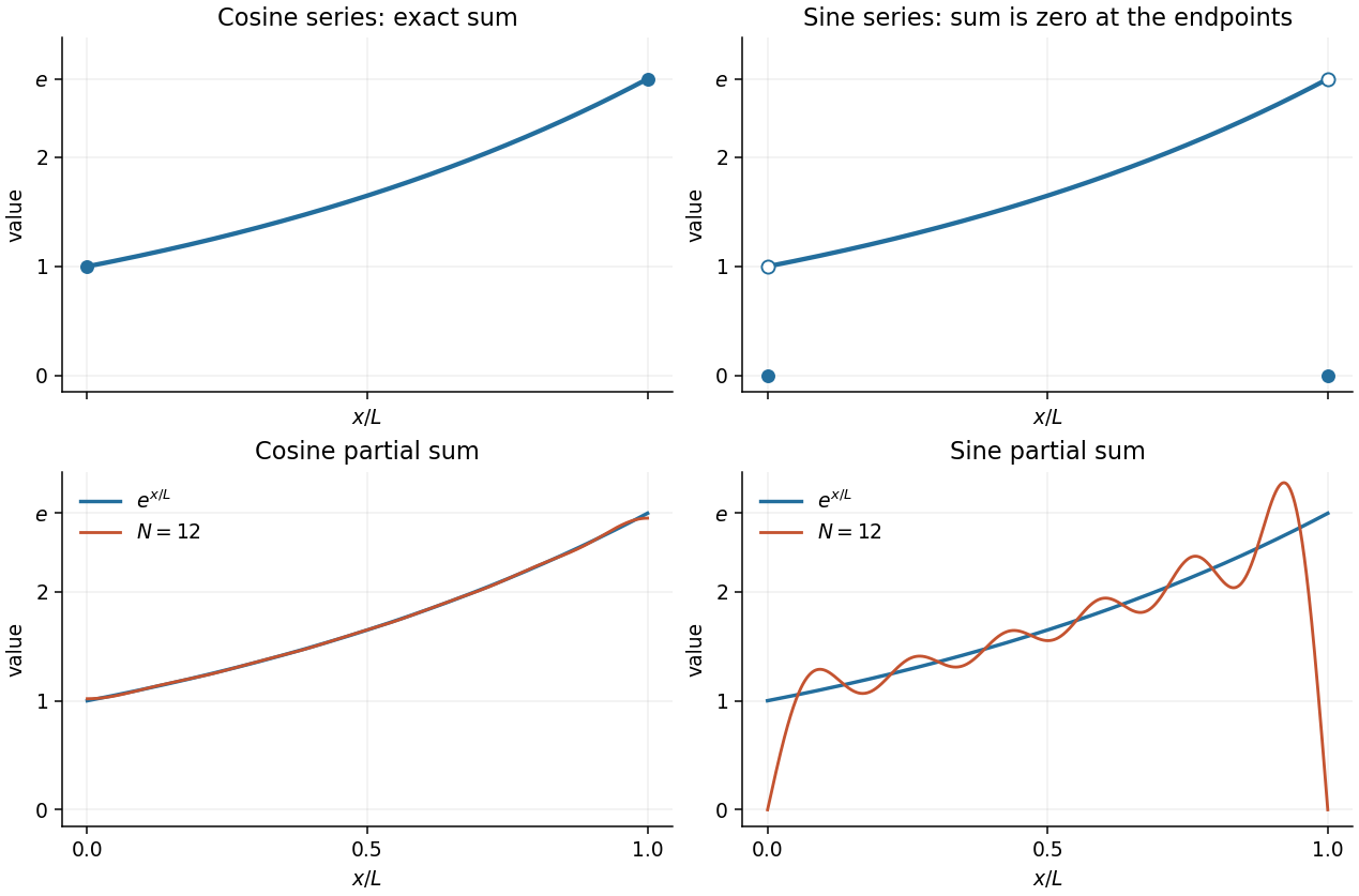
Under the stated piecewise smooth hypotheses, the Dirichlet convergence theorem for Fourier series gives the average of the two one-sided limits of the corresponding periodic extension. The even extension is continuous at both endpoints, so the Fourier cosine series converges toThe odd extension agrees with on , but its left and right limits are at zero and at the join . Therefore the Fourier sine series converges toIndeed every partial sum of the Fourier sine series is already zero at both endpoints. The endpoint values agree with only when the corresponding boundary values vanish.
The Fourier cosine series on isIt is the Fourier series of the even extension to , repeated with period . The Fourier sine series isIt comes from the odd extension and its -periodic extension. These Fourier coefficient formulas follow by Fourier orthogonality, since every nonconstant sine or cosine has squared integral on , while the constant function has squared integral .
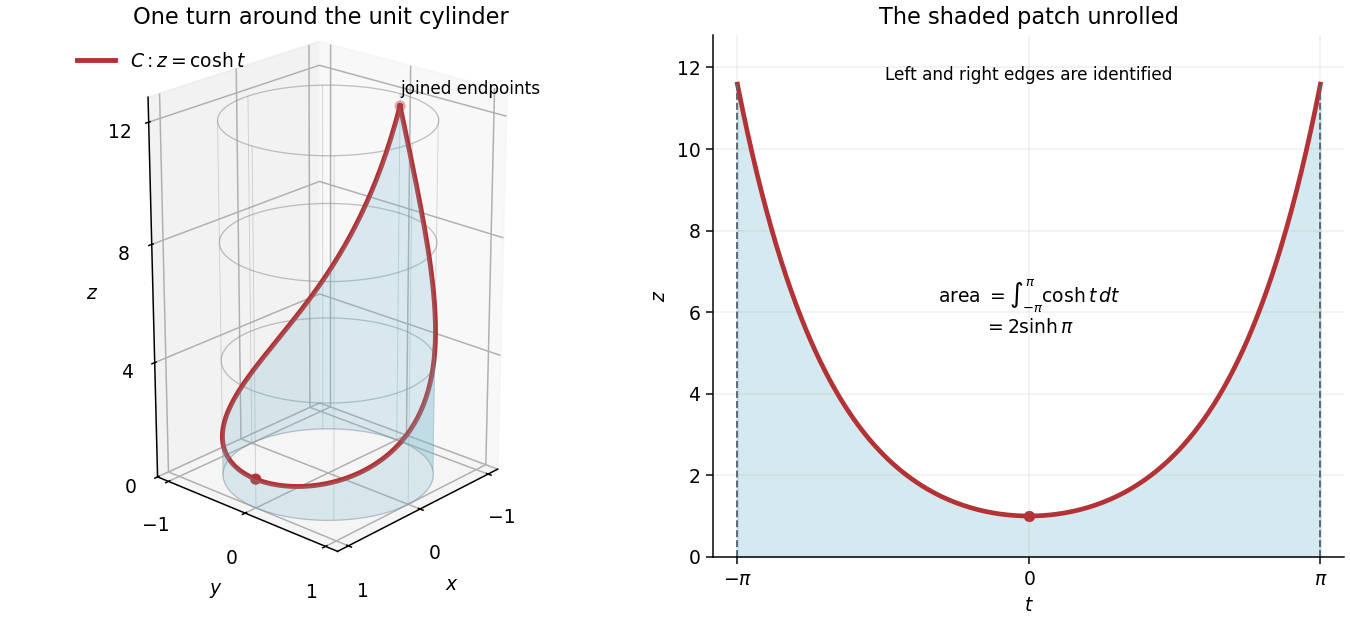
Parametrize the finite cylindrical surface patch byThe surface area element is . The seam has zero surface area, so it causes no overcounting. ThereforeUnrolling the unit circular cylinder preserves surface area, which explains the equality with the area under the hyperbolic cosine in the figure. The patch consists of the cylindrical surface alone; no flat base is included.
The velocity vector of the parametric curve isIts speed iswhere fixes the sign of the square root. Hence the arc length isThe coincidence of the endpoints does not duplicate any positive arc length.
For the given wrapped hyperbolic cosine curve,so . The curve makes one full turn around the circular cylinder, descending from to and ascending to its initial point. Its two parameter endpoints coincide; their tangent vectors and do not agree, so the resulting closed curve has a corner there.


True. Two applications of Green's identities, or two integrations by parts, giveThe biharmonic equation makes the left side zero, while the two clamped boundary conditions annihilate the boundary integral. Consequentlyso . Apply the first of Green's identities once more with : because on the boundary, it gives . By path connectedness, is constant, and the zero boundary value implies . This argument assumes the classical differentiability needed for the displayed integrations by parts.
There are unlisted articles, also show them or only show them.