
At any division step , an integer divides both exactly when it divides both : one direction uses , and the other uses . HenceStarting with , , the Euclidean division producesThe nonzero remainders form a strictly decreasing sequence of positive integers. Such a sequence must terminate, since there are only finitely many positive integers below . Suppose is the last nonzero remainder, so . The unchanged greatest common divisor at each step givesThe final equality holds because the positive common divisors of and are precisely the positive divisors of . This proves both termination and correctness of the Euclidean algorithm.
The divisions in the Euclidean algorithm areThe last nonzero remainder is , soAs a check, and ; back-substitution also gives .
At , the first three dual left sides are , and , strictly above their bounds , and . Thus complementary slackness forces . Both dual variables are positive, so both primal inequalities are equalities:Solving this linear system givesAll components are nonnegative, the two original upper bounds are met exactly, and the objective function equals the dual value. The weak duality bound therefore certifies optimality. The forced zero components and unique solution of the two remaining equalities also prove that the primal optimum is unique.
After removing the two redundant inequalities, the feasible region isIts lower boundary consists of three line segments or rays: for , then for , then for . The feasible region is everything on or above this boundary in the first quadrant.
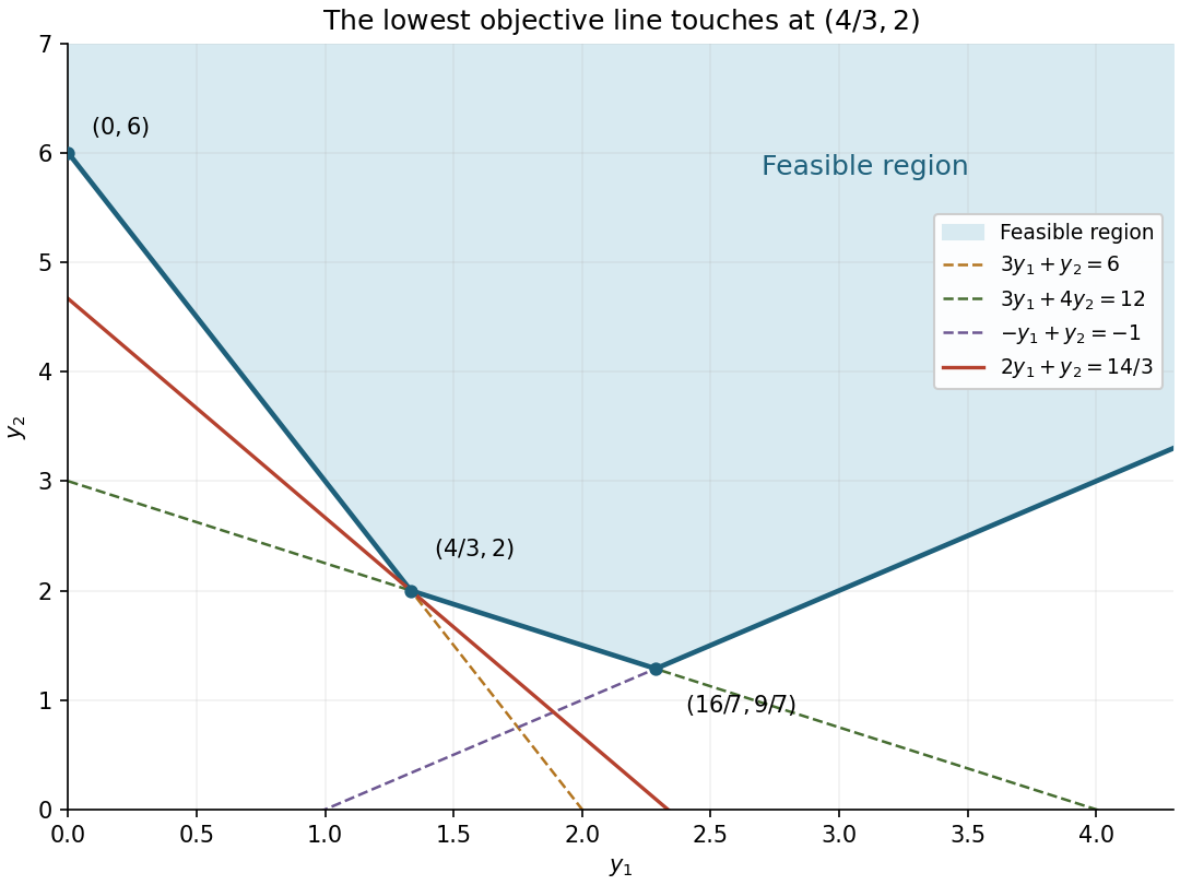

The boundary extreme points areAlong its three successive pieces, the objective function has respective slopes , and as increases. Thus it decreases to the middle extreme point and increases thereafter. For fixed , moving above the boundary only increases the objective function. HenceAs an algebraic check of the graphical answer, the active inequalities givewith equality at the stated extreme point.
The inequality , together with , impliesAlso impliesThus both inequalities are strictly slack throughout the feasible region. They are redundant: the remaining inequalities imply them, even with strict inequality. By complementary slackness, any primal optimum must therefore have ; this is the principle that strictly slack dual constraints force zero primal variables.
There are two primal inequalities, so there are two nonnegative dual variables. The five primal variables yield five dual inequalities:Each coefficient column of the primal linear program becomes one row of this dual linear program.
The complementary slackness conditions areTo see their role, decompose the duality gap asEvery summand is nonnegative for feasible solutions, so the gap is zero exactly when every displayed product vanishes. Zero gap implies optimality by weak duality. Conversely, strong duality states that primal and dual optima, when both are attained, have equal values, and hence satisfy these conditions.
For every primal feasible solution , weak duality givesThus no primal feasible solution improves on . Similarly, for every dual feasible solution ,Therefore both candidates are optimal, with the same objective function value. Equality is a linear programming optimality certificate and does not require a separate existence argument.
For feasible solutions , nonnegativity givesThe first inequality uses and ; the second uses and . This is weak duality.
If has rows and columns, attach a nonnegative dual variable to each of the upper-bound constraints. The dual linear program isHere is the transpose of , and all vector inequalities hold componentwise. Nonnegative dual variables preserve the direction of the original inequalities when taking weighted sums.
If , putThe linearized equation becomes , soArbitrarily small initial perturbations can have and grow exponentially. Hence the strict unstable equilibrium condition isFor the particular wire, this occurs precisely at , ; the alternating radii satisfy the stable equilibrium condition.
If , defineThe linearized equation is , with bounded simple harmonic motionThus the strict stable equilibrium condition isThis is also a sufficient condition for local nonlinear Lyapunov stability. Indeed the equation for the bead on a uniformly rotating wire has the conserved quantityIts derivative is times the governing equation moved to one side, so it vanishes. At , the last two terms have zero first derivative and positive second derivative . Their strict local minimum traps sufficiently small perturbations. The motion is bounded rather than asymptotically returning to rest.
Suppose a line through meets each . Its intersection with is different from , so lies in . A nonzero direction vector for must therefore satisfyA square matrix admitting a nonzero vector with has zero determinant. Expanding givesThus the necessary condition isThe condition is not sufficient. Take , which is on none of the three original lines. It satisfies the condition, since . The three plane equations becomeTheir common intersection is the single line . Any proposed line through meeting all three original lines would have to be this . But never meets : their second and third coordinates differ. The zero determinant guarantees a common direction for the three planes; it does not guarantee the required intersections. This is a parallel obstruction to a transversal of three skew lines.
The three lines have the convenient parametric equationsFor , substitute , in the plane through a point and a line given by a cross product formula. Its normal vector is . Cyclically permuting the coordinates gives all three planes:Each normal vector is nonzero because is not on the corresponding line. Thus these are genuine planes, and each is unique.
Apply the central limit theorem to the independent and identically distributed random variables , whose mean and variance are and . It gives the approximate standard normal distributionThe supplied standard normal quantile leaves probability in each tail. HenceSince , this event is equivalent toFor , equivalently integer , both denominators below are positive. Inverting the inequalities gives the approximate confidence intervalThe approximation is justified for large ; positivity at by itself does not guarantee accurate coverage. This construction is a confidence interval from a relative normal pivot: the unknown scale remains inside the pivotal ratio until the inequalities are inverted. Its meaning is that the random interval covers the fixed statistical parameter with probability approximately under repeated sampling.
The recurrence relation at gives . ConsequentlyBy variance additivity for independent random variables, the variance of their sample mean is
Be careful about the index: the probability density function already contains a factor , so . The recurrence relation at yields . Therefore linearity of expectation givesThus is an unbiased estimator.
For , the change of variables givesFor , use and integration by parts:The boundary term vanishes: at zero, and the exponential decay dominates the power at infinity. These estimates also establish convergence of the improper integrals used above.
For an observed random sample with all , which happens almost surely, independence gives the likelihood functionIgnoring a term independent of , the log-likelihood and its derivative areThis derivative is positive for and negative for . Thus there is a unique global maximum, and the maximum-likelihood estimator is
Assuming is measurable, applying it separately to independent and identically distributed random variables preserves those properties. Thus have common mean and variance . For , the central limit theorem givesHence, for large , the approximate probability distribution isThe second argument is the variance. If , this sample mean equals almost surely, so the appropriate description is a point mass at .
There are unlisted articles, also show them or only show them.