
For the mixed pair, and . The prescribed instantaneous orbital decay timescale givesThe integrated ten-billion-year merger criterion instead gives h. Both are pre-disruption circular-orbit estimates; the final contact/capture process differs from that for two neutron stars.
The binary of neutron stars has and . Inserting these into the circular orbital decay timescale givesUsing the integrated ten-billion-year merger criterion instead would give h.
Neutron-rich material ejected dynamically or in remnant-disk outflows can undergo the r-process: successive neutron captures, followed by beta decays, make heavy nuclei. The yield depends on the amount ejected, its entropy, expansion and electron fraction; not all outflow is equally neutron rich. Radioactive products can power a kilonova. A neutron-star–black-hole event contributes if matter escapes capture. An isolated binary black hole merger has no analogous reservoir of neutron-rich baryonic material, so it contributes essentially no such nucleosynthesis.
The changing mass quadrupole moment produces an inspiral gravitational wave signal whose frequency and amplitude increase toward merger. The chirp mass controls the leading frequency evolution, while higher-order phasing and the merger carry information about binary mass ratio and spins. Neutron stars also introduce tidal effects. These signals motivate a search with an interferometer such as LIGO; the supplied ranges quantify the paper's proposed detection prospects, without assuming any particular later observing-run performance.
A neutron star merger, or a neutron star tidally disrupted by a black hole outside its capture region, can leave a hot accretion disk around the remnant. Rapid accretion can power a relativistic jet and a short gamma-ray burst. Beaming means that an observer must lie sufficiently near the jet axis, and not every merger produces an observable burst. A clean binary black hole merger has no substantial baryonic fuel and is not ordinarily expected to power this mechanism. Disruption in a neutron-star–black-hole pair depends on binary mass ratio, black-hole spin and the neutron star's stellar radius.
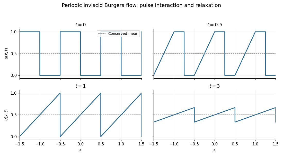
Let be the shock separating the fans from and . Their traces giveThus . Between consecutive shocks, . Writing for the fractional part, the period-one solution can be expressed, with right-hand shock traces, asTo put it in the requested fixed-support sum, takeThe half-open cells partition the line, so exactly one summand contributes at each point. This is a representation of the periodic solution, not a superposition principle for arbitrary solutions of a nonlinear equation.
The left and right shock states are and ; both average to the shock speed , and the strict inequalities certify causality. The periodic square-wave relaxation for the inviscid Burgers equation has the uniform estimateThe limit is the conserved mean .
For , translated copies of the preceding pulse have disjoint interiors of support. In the cell , write . The solution isAt use the given initial function. Each fan starts at , and each shock has position . At , the plateau disappears: its left fan catches its right shock at , which is also the starting edge of the next fan. The shocks must henceforth connect two nonconstant fan branches rather than a fan to a zero interval.
The initial condition is a period-one square wave: height one on each interval and zero on each gap , for integer . Each period has mean .

For the preceding sign convention, Green's second identity gives the harmonic representationprovided the far-boundary term vanishes or the bounded-solution representation applies. The face contributes nothing because . On , the outward normal is , so the remaining kernel is . Differentiating the image sum givesThus the requested constants areThe Poisson kernel of a three-dimensional quarter-space is the difference of the upper-half-space kernel and its reflection in . For bounded, suitably continuous data it produces the bounded harmonic solution, taking the prescribed traces away from the edge. Continuous data at the common edge must be compatible. Without any growth restriction at infinity, boundary values alone do not give uniqueness: a multiple of the harmonic function can be added while leaving both face values zero.
The supplied positive free-space kernel satisfies , so use the same sign convention for the Dirichlet Green function. For an interior source , requireAway from , the function is harmonic, and is regular near . The method of images reflects the source in each coordinate plane, reversing its sign on each reflection. ThereforeOn either face, the terms cancel in pairs. Only the original source lies in the domain, so the other three terms are harmonic there; the required singularity and decay also follow. This is the Dirichlet Green function for a three-dimensional quarter-space. Using instead would change the sign of the kernel and the representation formula together, as in sign conventions for a Dirichlet Green function.
Use the first order statistic and correct its bias:This is a measurable function of the sample. Under , write . It lies in , and independence givesFor a bounded nonnegative random variable, integrating the identities and proves the tail integral formula for moments by Tonelli's theorem. HenceThus is an unbiased estimator. Its quadratic risk is the variance of , independent of :Taking the supremum over all real and then the infimum over estimators givesThe final inequality follows from . Together with part (i), this proves that the minimax risk has order for all . In the last line of the source, the request for the upper-bound constant calls it ; here it is denoted consistently with the upper-bound inequality.
Use two translated uniform distributions, with parameters and . Their distance in the usual metric is , so take the separation radius and the loss function . The supplied testing reduction, equivalently the Le Cam two-point lemma, and part (a)(i) implyTo see the reduction directly, turn any estimator into a binary hypothesis test by choosing the closer of and . If the test is wrong, the absolute estimation error is at least . The worst quadratic risk is at least its average over these two parameters, giving precisely this bound.
Under Lebesgue measure on , the two sample probability density functions are the indicators of the cubes and . Their intersection is , of volume . Thereforewhere the inequality is Bernoulli's inequality. ConsequentlyThis also fits the Hellinger distance approach: the two one-sample affinities give , while equal-height indicator densities imply . Part (a)(ii) thus yields the same bound . The change of support produces Squared Hellinger distance proportional to , explaining the parameter scale and quadratic risk scale .
Put with the paper's normalized Hellinger distance. The Hellinger affinity isThe last bound follows from the Cauchy-Schwarz inequality and the unit integrals of the two probability density functions. Using a common dominating probability measure, for example , makes the product calculation immediate. The probability density functions of the product measures factor, and Tonelli's theorem givesThe Squared Hellinger distance is independent of the choice of common dominating measure, so this calculation applies to the original distributions. We obtain the exact identity and then apply Bernoulli's inequality:For completeness, the scalar bound follows by induction: , and multiplying by the nonnegative gives .
The statement necessarily treats as probability measures, as required by the sampling model . The word "measures" in the introduction must be read with this normalization. Use the paper's convention for the Squared Hellinger distance throughout this question.
A measurable binary hypothesis test is determined by the measurable set . Under the uniform prior on the two hypotheses, its error probability isSince the two measures have equal total mass,Indeed, the integral over any set is at most the integral of the positive part, and equality holds for . This is also the total variation distance. The likelihood ratio rule choosing hypothesis precisely on that set therefore attains the infimum, provingArbitrary choices on the tie set leave the error unchanged. This is the exact link between total variation distance and optimal binary statistical hypothesis testing.
Let be the eigenvalues of the positive-definite matrix . Its trace satisfiesThe arithmetic-geometric mean inequality givesSince , taking the logarithm provesThe determinant is largest, for a fixed trace, when the eigenvalues are equal; this is the geometric content of the estimate.
Work for an arbitrary realization of the sequence, and set . In the Loewner order,By the spectral theorem for real symmetric matrices, every eigenvalue of is at least . The matrix inverse therefore has eigenvalues at most , andFor , put . Since and , we have . The matrix determinant lemma now givesTaking logarithms and using a telescoping sum,This elliptical potential bound holds for every realization and every , without a probabilistic exceptional event. The condition is what ensures .
We give a finite chaining argument, keeping the constants explicit. If , the metric space has just the point and both sides vanish. Suppose , and writeChoose a smallest metric net of radius , and maps satisfying . Set and . Since is finite, choose with smaller than the minimum distance between distinct points; then and .
For each , retain only the pairs actually occurring along these approximation paths:The triangle inequality gives for ; for the same argument uses . AlsoHere only monotonicity in the radius for the same space is used. No monotonicity under subsets is assumed.
For every pair in , the increment has the Sub-Gamma random variable in the right tail bound with common parameters and : for ,Identical pairs give the zero increment, which obeys the same bound. Both orientations have finite exponential moments, so all increments are integrable random variables. Differentiating their two upper bounds at zero also gives . Applying the maximum bound from part (b), including its case, givesThe telescoping sum along each path is exact:Take the supremum, bound it by the sum of the maxima, and take expected values. This provesFor either or , the function is nonnegative and nonincreasing. ThusCombining the estimates yields the required metric entropy bound:In particular, and work. The square-root and linear metric entropy terms arise respectively from the two terms in the sub-Gamma maximum bound. Because the chain ends exactly at , no limiting sample-path regularity assumption is needed.
Use closed balls with centres belonging to the space being covered. The covering number iswith value if there is no finite metric net, and value zero for the empty space.
With this intrinsic-centre convention, the proposed monotonicity under subsets is false. Give the usual distance, take , and set . A ball centred at covers , so . The two points of are distance apart, so a ball centred in contains only its centre, and . These values are also valid with open balls.
The obstruction is that the useful centre disappears on passing to the subspace. If centres were allowed anywhere in a fixed ambient space, monotonicity would hold. With intrinsic centres, one instead hasIndeed, discard covering balls missing and choose one point of from each remaining ball. The triangle inequality shows that every point of its intersection with is within of the chosen point. This proves the replacement bound whenever the right side is finite; otherwise it is automatic.
Past exam of the algebraic number theory course of the University of Oxford 2023 2 b iii Solution 2026-10-25
The printed domain assertion is false. For example, take and . Then has the nonzero zero divisor , so it is not an integral domain and cannot be a principal ideal domain. The valid conclusion is that is a principal ideal ring. This error is present in the original PDF, not just its transcription.
To prove the corrected conclusion, factorinto powers of distinct nonzero prime ideals. These powers are pairwise comaximal ideals. Indeed, a maximal ideal containing two such powers would contain both underlying prime ideals, forcing them to be equal. The Chinese remainder theorem givesEvery factor is a principal ideal ring by the preceding part. Every ideal in a finite direct product of rings is a product of ideals in the factors: multiplication by the coordinate idempotent elements separates the coordinates of every element of . Write . Thenso is a principal ideal ring. This proves the principal ideal property of quotients of a Dedekind domain in the present setting. In fact, this finite quotient ring is an integral domain precisely when is a prime ideal, in which case it is a field.
For the final deduction, choose any and apply the result to the nonzero proper ideal . The ideal of is generated by one residue class , which can be represented by . For each , some satisfies . HenceThis proves two generators for an ideal in a Dedekind domain; moreover, its first generator can be any prescribed nonzero element of .
Past exam of the algebraic number theory course of the University of Oxford 2023 2 b ii Solution 2026-10-25
For every , the inclusion is strict: equality, followed by multiplication by the inverse of , would give . Hence one can choosePut . ThenThe classification just proved, applied modulo , leaves no ideal strictly between consecutive powers. It follows thatFor , the same argument says , using and maximality.
The extension to every follows by mathematical induction. Suppose . Multiplication of the initial equality by givesSubstitution yieldsThusTaking for givesThis is a principal ideal of the quotient ring . Its zero ideal is generated by zero, so every ideal of this quotient ring is a principal ideal.
There are unlisted articles, also show them or only show them.