
Set . The differential operator in the modified Helmholtz equation depends only on . Let be its decaying Green function. Acting on the proposed integral with the operator, in the sense of distributions, givesThe last step is the sifting property of the Dirac delta. ThusFor a regular rapidly decaying source, the singularity of the kernel found in part (ii) is locally integrable in three dimensions, and its convolution with the source tends to zero at infinity. This verifies both the equation and the decay condition. The sign of the kernel below corresponds to ; reversing the sign of the entire operator reverses the kernel.
Only two coefficients in the Sturm-Liouville eigenfunction expansion are nonzero: and . Since , the result of part (i) simplifies toUsing Parseval's identity, the prescribed weighted norm becomesThus , so or . Positivity selectsThe standing nonresonance assumption still applies: this answer requires that is not one of the unspecified higher eigenvalues. Their actual values are not supplied. If a higher eigenvalue were , the stated exclusion would fail and the data would not have an admissible under that exclusion.
Write in the complete Sturm-Liouville eigenfunction expansion. To determine , multiply the differential equation by and integrate. The Sturm-Liouville operator has the symmetry identitybecause both functions obey the homogeneous Dirichlet boundary conditions. Consequentlyso that . The stipulated exclusion of every eigenvalue makes all denominators nonzero, and givesThis is the resolvent operator applied to in the weighted space. The same projection shows uniqueness: a homogeneous solution would have for every , hence would vanish by completeness. For the regular problem the formula gives the solution in the operator domain when is square-integrable.
The path rises from to its maximum height at , then falls symmetrically to . Its radius is , and its endpoint polar angles are and , giving angular span . Hence its ordinary arc length isEquivalently, and integrating over gives the same value. This Euclidean length differs from the weighted destruction integral : the slightly longer route saves undergrowth by travelling at greater height.
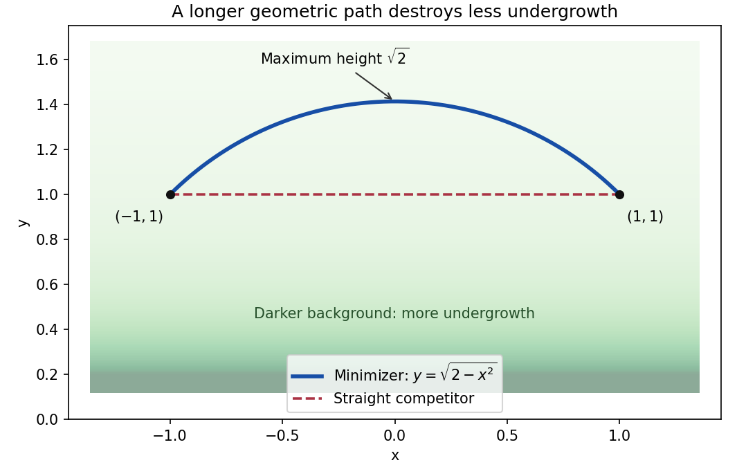
The least-destruction path bends towards lower density
. Original exact semicircular minimizer and its horizontal competitor. The shaded background indicates the density in the upper half-plane. The minimizer has Euclidean length but weighted cost , smaller than the straight path's cost two. Details.
Interpret the density on the physical region . It is singular at zero and would not describe a nonnegative density for . The first integral gives for a positive constant . To handle the horizontal tangent without dividing by , use the full Euler-Lagrange equation:Two integrations give . The equal endpoint heights force , and either endpoint then gives . ThusThe path is the upper circular arc. A constant horizontal path solves the differentiated first integral trivially but fails , so is not another extremum.
One can prove global minimality, rather than only stationarity. Define on the upper half-plane. ThenThe Cauchy-Schwarz inequality gives, along any admissible path from to ,Our circle has tangent for increasing , so equality holds pointwise. This calibration for semicircular hyperbolic geodesics provesThe geometry is that of a hyperbolic geodesic in the Poincaré half-plane model. The proof even allows competing upper-half-plane paths beyond the class of monotonic graphs.
The monotonic horizontal coordinate allows the path to be written as a graph. Its arc length element is , so the variational density is . It has no explicit horizontal-coordinate dependence. The Beltrami identity becomesConsequently every smooth minimizing path satisfiesThis is a first integral of the weighted arc-length problem; fixed endpoint values remove the endpoint variation terms.
Let . For every fixed real , the base is positive once is sufficiently large; any initial negative or zero bases affect only finitely many coefficients. For that tail,The Cauchy-Hadamard theorem therefore yieldsFor example recovers the geometric-series radius one. The stronger expansion also shows that, on , the magnitudes of the individual terms tend to . Thus this series diverges at every point on its convergence circle; the radius itself does not require that extra boundary analysis.
For coefficients , the Cauchy-Hadamard theorem gives . HereThereforeOmitting the first two powers has no effect on the radius of convergence.
Choose the common orthonormal eigenbasis established in part (ii), and let be the unitary matrix of its columns. ThenConsequentlyThus is unitarily diagonalizable, even though it need not be Hermitian. As a consistency check, commutation also gives , so is a normal matrix, as also follows from unitary diagonalization of a normal matrix.
Suppose first that , and take an eigenvector of , with . Commutation givesSince the eigenvalue is simple, its eigenspace is one-dimensional, so for some scalar . Thus every vector in an eigenbasis of is also an eigenvector of . The simple spectrum of ensures these account for its eigenvector directions as well. Eigenvectors are understood up to nonzero scaling and permutation, rather than as literally identical numerical vectors.
Conversely, if are a common eigenbasis with and , thenfor every basis vector. Hence . ThereforeThis is simple spectrum gives simultaneous diagonalization. Without simple spectra, commuting Hermitian matrices still possess a common orthonormal eigenbasis, but not every arbitrary eigenvector of one matrix must be an eigenvector of the other.
Using , the conjugate transpose of the proposed matrix isThusThe commutator of two Hermitian matrices is skew-Hermitian, and multiplication by changes it into a Hermitian matrix. No simplicity assumption on the spectra is needed for this part.
Use the branch from part (i) and close the real-axis path with a large upper semicircle, indenting clockwise around and . On the segment between them, take the upper-bank value of the branch cut. This is an instance of square-root endpoint integrals by an upper-half-plane contour.
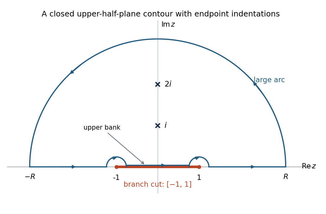
Upper-half-plane contour, clockwise endpoint indentations, and the two enclosed poles; indentation sizes are exaggerated
. Details. 
The contributions can be controlled separately. Since , the large arc contributes . Near either branch point, , so an arc of length contributes . On the upper bank of ,which is odd in , so its integral is zero. On the exterior real intervals , while the rational numerator is odd. Hence and the two exterior contributions sum to .
The rational factors give four simple poles at ; none is canceled by the numerator. The square root has branch points at , with local behaviour proportional to in the integrand.
For this part, choose analytic off and satisfying at infinity. Its values are for , for , andThus the chosen branch cut is , and the function is analytic elsewhere apart from the four poles. Infinity is not an intrinsic branch point: on this branch.
Another legitimate convention applies the positive-axis square root of part (a) to ; it places the cuts on and . Its upper-half-plane values agree with the branch used here, so the contour calculation below and the positive real square root in the required integral are unchanged. The branch choice must be stated because a square root alone does not specify a single-valued complex function.
For , the upper-bank argument tends to zero, whereas the lower-bank argument tends to . ThusThe analytic function has identical boundary values across this part of the real axis. Hence the branch cut introduces a sign change:This compares integrand values. When two contour segments traverse opposite banks in opposite directions, their orientation supplies an additional minus sign.
Choose , so on the arc. Its clockwise orientation givesBecause is an analytic function at zero, uniformly on the small arc. Integration then givesThereforeThe estimation lemma also gives . Hence a sufficient large-arc condition isFor example uniformly on the arc, with , suffices. Under the stronger literal assumption that is analytic at infinity, its Laurent expansion is ; the necessary and sufficient condition is then . A nonzero constant term would instead give the growing contribution .
Write , . For a spherical source, the angular integral needed for the Green function of the Laplacian isThis is the angular form of the spherical shell theorem. Substituting the source into the Green function integral therefore yieldsThe elementary integrals areThe terms proportional to cancel, leavingThe value at the origin is the continuous limit. At large radius , consistent with the integrated source and the factor in the far-field potential.
For a direct check, set . Then , so for . Boundedness of at zero cancels the singular terms and excludes an extra point source. The original density is itself singular but locally integrable; the equation at the origin is understood in the sense of distributions. This is the Poisson potential of an exponential-over-radius source with amplitude .
Translation and rotation invariance allow a radial Green function , with . Outside the source, , so . Decay at infinity gives .
Integrate the defining equation over a small ball centred on the source. The divergence theorem fixes its flux:ConsequentlyThis is the Green function of the Laplacian with the stated negative-delta sign. A homogeneous addition would change the delta normalization, so the singular coefficient is fixed, not an arbitrary integration constant.
Define the candidate potential by convolving the decaying Green function with the source. Acting with the Laplacian in the observation variable gives, in the sense of distributions,The final equality is the sifting property of the Dirac delta. The kernel found in part (ii) is locally integrable, and its convolution with a sufficiently regular rapidly decaying source also vanishes at spatial infinity. Thus it satisfies the Poisson equation and the required condition at infinity.
The difference from any other regular decaying solution is a harmonic function on all of space vanishing at infinity, hence is zero by the maximum principle. ThereforeOne can also obtain this expression from Green's second identity on larger and larger balls, with the singularity of the kernel treated distributionally. The surface term at infinity vanishes for the usual potential decay and gradient decay.
Equal endpoint heights implyso . The height condition then gives and the hanging catenary isSince , its length fixes throughFor the requested graphical argument, put and . Intersections of with determine the solution. Near zero the line has larger slope, while the hyperbolic sine eventually grows faster. Its slope increases strictly, so after turning upwards relative to the line it can cross it only once. The intersection at is excluded: it corresponds to infinite and the limiting length .
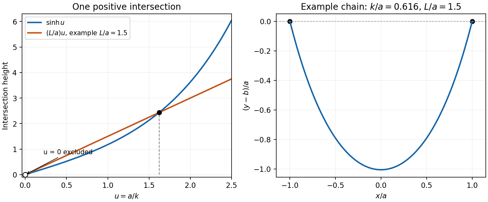
Unique positive catenary parameter from a hyperbolic-sine intersection, with an example hanging chain
. Details. 
More explicitly, has derivative , because the numerator vanishes at zero and has derivative . Since and , every yields exactly one positive , hence exactly one positive .
Introduce a constant Lagrange multiplier for the fixed arc length. Up to an irrelevant constant term, the augmented functional isIt has no explicit dependence, so the Beltrami identity givesFor the hanging minimum choose . Writing , this becomes . Its nonconstant smooth solution isOne may verify it without dividing by at the lowest point: the full Euler-Lagrange equation gives , which the expression satisfies everywhere. The branch with negative is the inverted stationary chain rather than the hanging minimum. The catenary minimizes the integral of height along a fixed-length curve, so the positive branch is also the global minimum, not merely a stationary candidate.
There are unlisted articles, also show them or only show them.