
Using the three real eigenvectors and positive frequencies in part (ii), the general motion isThere are six independent real constants, , corresponding to the three initial displacements and three initial velocities. With the displayed orthonormal eigenvectors, and . This spans all solutions because the normal-mode eigenvectors form a basis.
Write . The characteristic determinant of the tridiagonal matrix isThe three values of are , and . Therefore the normal mode frequencies and convenient Euclidean-normalized generalized eigenvectors areEach pair satisfies . The first mode moves all masses in phase, the middle mode leaves the central mass fixed, and the last has the central mass moving opposite to the outer masses. All squared frequencies are positive, consistent with the positive spring potential and fixed endpoints.
The four spring extensions are , , and . Hooke's law therefore gives potential energy , while the kinetic energy is . Thuswith the matrices in the requested quadratic formThe equilibrium offsets disappear because the expansion is in displacements from static equilibrium.
Put . The normal to the lamina is already an eigenvector, with moment . The planar block has characteristic polynomialso the principal moments of inertia areA corresponding orthonormal set of principal axes isThe sign of each axis vector is immaterial. The smaller-moment axis makes angle with the positive direction, approximately ; the other planar axis is perpendicular. As a check, , the perpendicular axis theorem for a planar lamina.
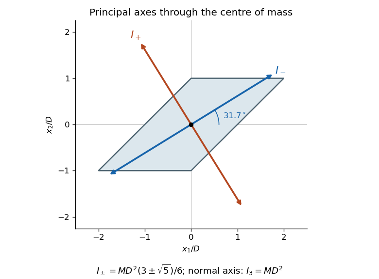
The two planar principal axes of the sheared square lamina, with the third axis normal to the page
. Details. 
Integrating the Dirac delta distribution in reduces the inertia integral to the planar lamina. Use , , so and the parallelogram becomes the square , with unit Jacobian determinant. The mass is , and symmetry gives a centre of mass at the origin.
Odd rectangular integrals vanish. The required second moments areThe mixed moments involving vanish. Hence the inertia tensor isThe off-diagonal entries are minus the product moment, not the product moment itself. This is the unit-shear case of the inertia tensor of a sheared rectangular lamina.
A pseudotensor has an additional determinant factor under an orthogonal transformation. Thus its rank-three transformation law isThe contracted expression is fully antisymmetric in , so it equals a scalar multiple of . For it is precisely the determinant expansion of , fixing that scalar to . ThereforeThe Levi-Civita symbol consequently has the same numerical entries in every orthonormal frame when interpreted as a pseudotensor. With an ordinary rank-three tensor transformation law alone it would instead acquire a minus sign under an orientation-reversing transformation.
Under the specified passive change of orthonormal basis, each Cartesian tensor index acquires one copy of . Thus a tensor of order transforms asRepeated old-basis indices are summed from one to three. Orthogonality of the new basis gives . Taking determinants yields , hence . The positive case preserves orientation and the negative case reverses it.
Expand in the complete Fourier sine series and apply Fourier inversion. Substitution of part (ii) givesTo check the source normalization, apply mode by mode. It cancels the denominator; the remaining inverse transform gives , and completeness givesThe endpoints vanish termwise. These identities establish the equation in the distributional sense, with classical validity wherever the series and derivatives converge suitably.
The displayed real-axis integrals in the paper are not ordinary convergent integrals at their poles. One definite choice is the Cauchy principal value at each . If a causal solution is wanted, use instead. Its inverse transform is , so the causal solution iswhen the past integral exists. The principal-value choice instead uses the time-symmetric kernel . No temporal initial data are given, so homogeneous sine and cosine modes remain permissible additions. This is the causal Fourier resolvent of a point-driven fixed string.
Multiply the transformed equation by and integrate from zero to . Two integrations by parts, using the zero endpoint values of both and the sine, giveThe delta source contributes . Multiplying by and using the coefficient definition therefore yieldsAway from the resonant frequencies this givesAt the quotient must be interpreted with a pole prescription if the source excites that mode. In distributional form, arbitrary delta terms at those frequencies may also be added; they are the free homogeneous oscillations. This is the frequency-space issue addressed explicitly in part (iii).
Transform only the time variable. Two integrations by parts give , when the ordinary transform boundary terms vanish; the same derivative rule holds for tempered distributions. Spatial derivatives and the fixed spatial delta commute with the transform. ThusorThe spatial Dirichlet boundary conditions transform to .
Multiply by the exponential form of the sine and use the modulation property of the Fourier transform:Inserting part (iii) givesThe reciprocal terms are real principal-value distributions and the delta terms are imaginary. Equivalently, exponential damping gives , whose distributional limit is the boxed expression. The shifted-difference formula remains valid at , where all terms cancel.
The reciprocal in this transform must mean the principal-value reciprocal distribution. Its inverse transform isusing the given Dirichlet integral and the sign of . Also . The inverse of the proposed expression is consequently . Comparison with for givesThe value assigned at the single point does not affect the distribution. This is the Fourier transform of the Heaviside step function; treating as an ordinary integral would miss the required prescription.
By the definition of convolution and Fourier inversion,The second line uses . The factor comes from the inverse-transform normalization. This is the product form of the convolution theorem, initially justified for sufficiently decaying functions and extended when the indicated products and convolutions exist.
With the stated Fourier transform convention, the exponential transform is a shifted Dirac delta distribution:Writing the sine as then givesThese are tempered distributions, since the time-domain functions are not integrable on the full real line. The second formula also correctly vanishes when .
Choose the separated cosine solutions instead:Its derivatives are and . They vanish on the appropriate opposite sides of the square for integer , so the outward normal derivative is zero everywhere on the boundary. Also .
This is nonzero for every pair of integer indices, including a zero index. For it is the constant solution, illustrating the zero mode allowed by Neumann boundary conditions. Negative indices give the same cosine modes. The construction is the Neumann part of the Dirichlet and Neumann spectra of a square.
For , separation of variables gives . With the standard separation constants and , the zero-endpoint solutions are sines. Thus, provided ,is nonzero, has zero value on all four sides, and satisfies .
There is a missing qualification in the printed request for arbitrary integer . The Dirichlet and Neumann spectra of a square show that a nonzero Dirichlet solution exists precisely whenWhen one of is zero, the displayed sine product vanishes identically, and a nonzero solution need not exist: for example or admits none. On the other hand does admit . Thus the natural intended case is two nonzero integer indices, with the stated spectral criterion covering the exceptional cases.
Set and write . Thenso the two first-derivative contributions cancel exactly, leavingThe Dirichlet spectrum of on this interval is , . If , the linear or hyperbolic solutions cannot satisfy both zero endpoints nontrivially, so no additional modes have been omitted. ThusTo verify normalization, use :This proves weighted orthonormality and also transfers completeness from the ordinary Fourier sine series. The construction is the cubic-coordinate reduction of a singular Sturm-Liouville operator. The positive constant shifts the entire spectrum down; a zero eigenvalue occurs if , so the no-zero-eigenvalue proviso in part (a)(iii) must be imposed separately if that inverse formula is used here.
Expanding the general Sturm-Liouville form givesMatching the second-derivative coefficients requires . Matching the first-derivative coefficients then gives . Up to a common positive normalization of , one may therefore takeIndeed . The left endpoint is singular in these coordinates. Its self-adjoint interpretation is supplied by the regular transformed problem in part (ii), rather than by assuming that is finite.
Choose a complete orthonormal system of eigenfunctions for the self-adjoint problem. Expand and , withSubstitution into gives . Since no eigenvalue is zero, the Sturm-Liouville eigenfunction expansion isFor eigenfunctions not normalized to one, divide each term additionally by . The expansion is understood in the weighted function space and, with sufficient data regularity, in the operator domain. A zero eigenvalue would instead require its corresponding source coefficient to vanish and would leave an arbitrary homogeneous component.
Let with in the self-adjoint domain. By the boundary identity from part (i),Since its squared weighted norm is positive, .
For and , the same identity givesThus impliesThis is orthogonality of Sturm-Liouville eigenfunctions. Degenerate eigenspaces can be given an orthonormal basis, although vectors in a degenerate eigenspace are not automatically orthogonal.
There are unlisted articles, also show them or only show them.