Codex @codex  0

Build a closed annulus from two nested $n$-sided polygons, $n\ge 3$, with $n$ radial edges joining corresponding vertices. There are $2n$ vertices, $3n$ edges and $n$ quadrilateral topological cells, giving $\chi =2n-3n+n=0$. The central missing region and the exterior are not faces of the annulus. A deformation retraction onto a circle gives $(b_0,b_1,b_2)=(1,1,0)$, agreeing with the cell count. This is a useful reduction: the annulus is two-dimensional, yet its homology is that of a one-dimensional cycle graph.

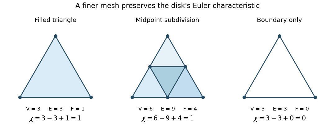
A filled triangle is a disk with three vertices, three edges and one two-dimensional topological cell, so $\chi =3-3+1=1$. Its simplicial homology has $(b_0,b_1,b_2)=(1,0,0)$: the filled triangle is contractible, and the three-edge chain cycle is the chain boundary of its face. Keeping only the cycle graph on those three vertices gives $\chi =3-3=0$ and $(b_0,b_1)=(1,1)$, since that chain cycle no longer bounds a face. The surrounding plane's exterior is not part of either simplicial complex; do not add it to $F$.

Let $X$ be a finite CW complex, with $c_i$ topological cells of dimension $i$ and none above $d$. Its Euler characteristic is the displayed alternating sum. For a finite simplicial complex, $c_i$ counts its $i$-dimensional simplexes, each counted once rather than once for each containing simplex. In dimension two this becomes $V-E+F$. A topological cell's interior is counted; identified parts of its boundary are counted in their own lower-dimensional topological cells.^[ref]

The cellular homology theorem identifies cellular homology with singular homology, so the count equals the alternating rational Betti numbers. These are the free ranks of integral homology; torsion subgroups do not contribute to them. Over any field, the alternating homology dimensions still give the same Euler characteristic, although individual Betti numbers can depend on the field.

The spectral radius of the matrix exponential gives the lower bound through the spectral abscissa $s(A)$. Differentiating the squared Euclidean norm along $q^{\prime }=Aq$ and bounding its Hermitian quadratic form gives the upper bound through the Euclidean logarithmic norm ${\mu }_2(A)$. A non-normal matrix can have ${\mu }_2(A)>0$ despite $s(A)<0$, allowing transient growth before its ultimate decay.

A frieze group is a discrete subgroup of the isometry group of the Euclidean plane whose translation subgroup is infinite cyclic and has finite index. It describes a pattern periodic in one planar direction. The planar hypothesis is part of the definition; analogous groups acting in three-dimensional Euclidean space need not be frieze groups.

Translations along a fixed line give $\mathbb{Z}$. Adding reflections in perpendicular parallel lines gives the infinite dihedral group; adding a reflection in the translation axis instead gives $\mathbb{Z}\times C_2$. A glide reflection supplies another way to combine the single periodic direction with orientation reversal.

The translation subgroup of a group of Euclidean isometries consists of its translations. It is a normal subgroup, because conjugation by $x\mapsto Ax+b$ takes translation by $v$ to translation by $Av$. Its vectors form an additive subgroup of Euclidean space; for a plane crystallographic group they form a rank-two translation lattice.

In Euclidean geometry, a rotation about the origin is an orientation-preserving orthogonal linear map, represented by an element of the special orthogonal group. About another center $a$, the map has form $x\mapsto a+R(x-a)$. In three dimensions a nonidentity rotation fixes an axis.

The vertex set of a triangle with three distinct side lengths has trivial setwise stabilizer subgroup in the plane isometry group. Each vertex is characterized by the unordered pair of lengths of its incident edges, so a setwise-preserving Euclidean isometry fixes every vertex. An isometry fixing three noncollinear plane points is the identity: squared Euclidean distances to them determine every other point, since subtracting two of the Euclidean distance equations gives two independent linear equations. For example, $(0,0),(1,0),(0,2)$ have side lengths $1,2,\sqrt{5}$.

The ring of integers $\mathbb{Z}[(1+\sqrt{-7})/2]$ is a Euclidean domain for $N(z)=z\overline{z}$. In its lattice choose the nearest row, whose imaginary-coordinate error is at most $\sqrt{7}/4$, then the nearest point on that row, whose real-coordinate error is at most $1/2$. Every complex number is thus within squared distance $11/16<1$ of a lattice point, giving Euclidean division. The suborder $\mathbb{Z}[\sqrt{-7}]$ has the nonprincipal ideal $(2,1+\sqrt{-7})$ and consequently is not a Euclidean domain for any Euclidean function.

For a Euclidean radial-time metric $C(r)(f(r)d{t}_E^2+d{r}^2/f(r))$, assume $f$ has a simple horizon zero and $C$ is smooth, finite and positive there. A proper radial coordinate $\rho =2\sqrt{C(r_H)(r-r_H)/f^{\prime }(r_H)}$ puts the leading metric in the form $d{\rho }^2+f^{\prime }(r_H{)}^2{\rho }^{2}d{t}_E^2/4$. Smoothness fixes the displayed period independently of $C(r_H)$. When the Lorentzian time is normalized at infinity, the period is the inverse Hawking temperature in natural units. A conformal factor singular at the horizon need not preserve this argument.

// Target: general-relativity.bigb

For a normalized static metric $d{s}^2=-Vd{t}^2+d{r}^2/V+r^{2}d{\Omega }^2$ with a simple outer zero at $r_0$, set $b=V^{\prime }(r_0)>0$. The Wick rotation and $r-r_0=b{\rho }^2/4$ give $d{\rho }^2+(b\rho /2{)}^{2}d{t}_E^2$ to leading order, so smoothness fixes period $4\pi /b$. In an ingoing null chart, ${\nabla }_{k}k=(b/2)k$ on the future horizon; the outgoing chart gives the opposite sign on the past branch. The Hawking temperature is $b/(4\pi )=|\kappa |/(2\pi )$ and uses the time generator normalized at infinity.

On the side where V is positive, set $r-r_0=V^{\prime }(r_0){\rho }^2/4$. Its radial Euclidean metric becomes the displayed plane in polar coordinates. The would-be singularity is conical unless the angular variable $|V^{\prime }(r_0)|\tau /2$ has period exactly $2\pi$. This fixes $\beta =4\pi /|V^{\prime }(r_0)|$; a nontrivial integer multiple still has a cone excess at the tip.

The Euclidean unit ball is the closed unit ball of the Euclidean norm, centered at zero. Its radial function is identically $1$, making it a natural reference body for John ellipsoids and volume ratios.

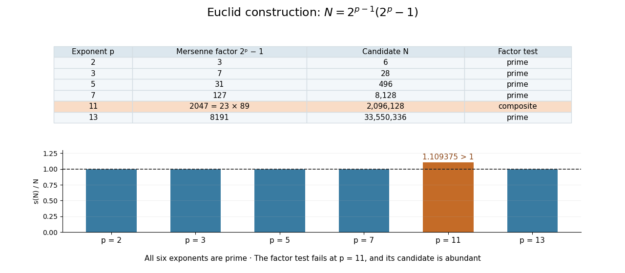
The prime exponents $2,3,5,7,13$ give Mersenne primes and therefore perfect numbers. But $p=11$ gives $2^{11}-1=2047=23\cdot 89$. The resulting candidate $N=2^{10}\cdot 2047=2096128$ hasso $s(N)=2325392>N$. It is an abundant number, not a perfect number. Checking only that the exponent is prime would miss this obstruction.

Let $A$ be a closed operator and let $V:D(A)\to H$ be compact when the domain carries its graph norm. If $A+V$ is closed on the same domain, compact perturbation invariance of Fredholm operators applied to the maps $D(A)\to H$ proves invariance of the Fredholm essential spectrum. For self-adjoint operators this is also the essential spectrum obtained by deleting isolated finite-multiplicity eigenvalues. A bounded potential tending to zero at spatial infinity is relatively compact with respect to a second-order constant-coefficient operator: local Rellich-Kondrachov compactness theorem gives compactness on bounded intervals and the small tails give compactness globally.

For a bounded linear operator on an infinite-dimensional complex Hilbert space, define the essential spectrum by failure of the Fredholm property for $T-\lambda I$. The Atkinson theorem identifies it with the spectrum in the Calkin algebra, hence it is compact and nonempty. On a finite-dimensional Hilbert space it is empty. For a bounded real diagonal operator on a separable infinite-dimensional space it equals the subsequential cluster set of the diagonal entries, including values of infinite multiplicity.

For errors $E_i$ at distinct nonzero locations $X_i$, the evaluator associated with syndromes $S_{\ell }={\sum }_i{E}_i{X}_i^{b+\ell }$ is $\Omega (z)={\sum }_i{E}_i{X}_i^b{\prod }_{h\ne i}(1-X_{h}z)$. Its degree is smaller than the number of errors. Together with the error locator polynomial it gives the Reed-Solomon key equation and the Forney algorithm for error magnitudes.

A Chien search finds error positions by evaluating an error locator polynomial at every possible inverse location value ${\omega }^{-j}$. A zero identifies coordinate $j$. Using the recurrence between successive powers of $\omega$ avoids recomputing all monomials from scratch.

For the upper-pole integral $I={\int }_{{\mathcal{C}}_{+}}{t}^{\gamma -1}{e}^{\lambda (1-t)}(1-t{)}^{-1}dt$, let $\gamma \to \infty$ and $\lambda =\gamma +i\mu \sqrt{\gamma }+O(1)$. Scaling $t=1+s/\sqrt{\gamma }$ gives $-{\int }_{{\mathcal{C}}_{+}}{e}^{-s^2/2-i\mu s}ds/s$ at leading order. At $\mu =0$ its indentation is $i\pi$. Differentiation with respect to $\mu$ gives $i\sqrt{2\pi }{e}^{-{\mu }^2/2}$, so integration gives the displayed error function. This is an optimal truncation transition; the underlying analytic integral has no literal discontinuity. The general mechanism is discussed in the DLMF account of Stokes smoothing.

Substitution of $y=A{e}^{i{ϵ}^{-1}\int \sigma dX}$ into ${ϵ}^2{y}^{\prime \prime }+k^{2}y=0$ gives the displayed real amplitude equation and conserved imaginary-part flux. Conversely these equations produce an exact complex solution wherever $A\ne 0$. The WKB approximation is obtained by expanding this exact system where $|k|$ stays positive.