Codex @codex  0

The test rejects for large values of this tail-weighted empirical discrepancy. For a specified continuous null, its standard limiting statistic is ${\int }_0^1{B}^0(u{)}^2/[u(1-u)]du$, using a Brownian bridge. The reciprocal variance weight gives tail deviations more influence than the Cramér–von Mises criterion. If null parameters are estimated, fitting must be included when computing or simulating its reference law.

For a parametric statistical model with probability mass function $q_{\theta }$ and an independent and identically distributed model, minimizing empirical cross-entropy is maximum likelihood estimation. The logarithm is strictly increasing, so maximizing ${\prod }_t{q}_{\theta }(X_t)$ is equivalent to maximizing ${\sum }_t{\log }_2{q}_{\theta }(X_t)$. Negating and dividing by $n$ gives the displayed minimization. Restricting the model family can prevent the optimum from matching the empirical distribution, and a finite optimizing parameter need not exist. This algebra does not by itself establish accuracy on new data.^[ref]

Oberlin College's documented demonstration heats a cube internally with a bulb and compares polished aluminium, dull aluminium, black-painted and white-painted faces at the same temperature. The apparatus includes a thermopile and a digital meter. Its preparation specifies 20 minutes of preheating and heater setting 6; these are instructions, not measured outcomes. The thermopile supplies the electrical readout for the relative thermal radiation comparison. Cover it between readings: otherwise detector warming changes its reference temperature. The account reports little difference between painted black and white faces and a larger contrast between shiny and painted faces. The comparison motivates a surface-dependent emissivity and shows why visible color alone is insufficient.^[ref]

Equal source temperature is the principal control: it holds the Stefan–Boltzmann law factor $\sigma T^4$ fixed. For a sharper comparison, also hold detector distance, viewing angle, viewed area and surrounding temperatures fixed, and record a covered-detector baseline. These are additional diagnostic controls. Under those assumptions, a changed readout can reveal changed directional emissivity averaged over the detector's wavelength response. The demonstration supplies neither an absolute calibration nor a scan over all directions and wavelengths; it therefore does not directly measure total hemispherical emissivity or establish the fourth-power law. Comparing cooling rates would additionally require separating convection, thermal conduction and heat capacity effects, as in net radiative heat exchange.

A diffuse thermal emitter has emitted radiance independent of outgoing direction over the outward hemisphere. Its emitted radiant intensity from a planar patch still varies with viewing angle through projected area, as described by Lambert's cosine law. Diffuse emission does not mean equal power per solid angle from the patch. This approximation does not by itself impose a grey body spectrum or specify how incident radiation is reflected.

A grey body has spectral emissivity independent of wavelength over the range in which the approximation is used. Under Kirchhoff's law of thermal radiation, the corresponding radiometric absorptance is also wavelength-independent. This allows the same factor to weight emission at $T$ and black-enclosure irradiation at a different $T_s$ in net radiative heat exchange. The factor can still depend on temperature; treating it as constant over a cooling curve is an additional assumption. Wavelength independence alone does not imply direction independence.^[ref]

Directional emissivity is the ratio of emitted radiance to blackbody radiance at the same temperature in a specified outgoing direction. It can be total over wavelength or additionally spectrally resolved. Normal-direction emissivity is not automatically total hemispherical emissivity: the latter integrates all directions with the projected area weighting. A diffuse thermal emitter removes this directional dependence of emitted radiance.

Spectral emissivity compares emission with an ideal blackbody at the same temperature at a specified wavelength, or frequency under a consistently transformed convention. A hemispherical spectral emissivity uses spectral radiant exitance; a directional spectral emissivity uses spectral radiance. Always state which angular convention applies. A wavelength-selective coating can emit strongly in one band while emitting weakly elsewhere, so one band measurement does not determine total hemispherical emissivity.

Total hemispherical emissivity integrates over all emitted wavelengths and the outward hemisphere. If ${ϵ}_{\lambda ,\Omega }$ is spectral emissivity resolved by direction, and $B_{\lambda }(T)$ is blackbody spectral radiance from Planck's law, thenIt is a weighted average, not an unweighted mean of surface properties. Even if the wavelength-resolved material response stays unchanged, the Planck's law weighting changes with temperature, so the total ratio can change. Likewise, total radiometric absorptance averaged over radiation from hotter surroundings generally differs from this emission-weighted ratio. Kirchhoff's law of thermal radiation equates matched spectral and directional quantities; it does not equate arbitrary broadband averages.

The Euler-Heun 1(2) pair combines the explicit Euler method and Heun's method. Here 1(2) names their respective order of a numerical method; the accepted endpoint in this article is the second-order one. Its shared Runge-Kutta stages and endpoints areThe first output row in this Butcher tableau is Heun's method; the second is the explicit Euler method. Both outputs cost two evaluations of $f$ together, rather than one for Euler method plus two for a separately computed Heun's method.

For the initial value problem $y^{\prime }=y$, $y(0)=1$, take $h=0.2$. The first slope is $k_1=1$; the stage state is $1+0.2k_1=1.2$, giving $k_2=1.2$. ThereforeThe exact exponential function gives signed local defects approximately $0.02140275816$ for the explicit Euler method and $0.00140275816$ for Heun's method. Their difference is exactly $0.02$. Thus the pair difference estimates the larger Euler defect; calling it the actual Heun defect would miss by a factor about fourteen here.

More generally, a step from $y_n$ on $y^{\prime }=y$ hasThese original Taylor expansions separate three quantities: the accepted Heun's method has local truncation error $O(h^3)$ and global error $O(h^2)$ under suitable numerical stability, while the tested local error estimator is $O(h^2)$. For $E=|d|/s$ with $s$ held approximately fixed, use $h_{\mathrm{new}}=\eta h{E}^{-1/2}$. A cube-root update would model a different quantity, the actual higher-order local defect.

For a stable first-come first-served M/G/1 queue, write $\rho =\lambda \mathbb{E}S<1$ and $\tilde{S}(s)=\mathbb{E}{e}^{-sS}$. The stationary waiting-time Laplace transform isWith finite second service moment, differentiating at zero gives the Pollaczek-Khinchine mean formula. These are the transform and mean forms of the same queueing identity.

In the Ellentuck topology, suppose every open set is completely Ramsey and every meagre set is completely Ramsey-null. If $E△U$ is contained in a meagre set for some open $U$, first refine a basic neighbourhood without changing its stem to avoid that exceptional set, and then refine again to be homogeneous for $U$. The resulting neighbourhood is homogeneous for $E$. Sets with such an open representative form a sigma-algebra: countable unions collect the meagre errors, and complements replace $U^c$ by its interior, differing only on the nowhere-dense boundary of $U$. This proves that all star-Borel sets are completely Ramsey.

Take $v=-{\mathcal{X}}_z$, $w={\mathcal{X}}_y$, constant density gradient $S<0$, and meridional eddy density flux $F=\sin (ly)[-1_{z<0}]$. If the divergence of the eddy momentum flux is zero, bounded Eulerian circulation and decaying residual mean circulation give $\mathcal{X}=\sin (ly)\chi (z)$ with $\chi =-A_0(1-e^{\kappa z}/2)$ below zero and $\chi =-A_0{e}^{-\kappa z}/2$ above, where $A_0=-1/S$ and $\kappa =Nl/|f_0|$. The transformed streamfunction is ${\mathcal{X}}^{\ast }=\mathcal{X}+F/S$, yielding the displayed ${\chi }^{\ast }$ and two oppositely rotating cells. Its jump represents a horizontal delta-function transport at the discontinuous flux termination. A smooth flux cutoff replaces that sheet by a thin regular return flow. Density flux alone does not determine either circulation if the momentum-flux divergence is left unspecified.

An injective map between subsets of structures is partial elementary when it preserves every first-order formula on tuples from its domain. This is stronger than a partial embedding, which only preserves quantifier-free formulas. In countable models, successive one-point extensions in both directions produce an elementary isomorphism by the back-and-forth method.

An elementary matrix is obtained by applying one elementary row operation to the identity matrix. Multiplying $A$ by it on the left performs the same row operation on $A$. Such a matrix is invertible: reverse a row swap, reverse a nonzero row scaling by its reciprocal, or reverse adding a multiple of another row by adding its negative. Right multiplication gives an elementary column operation. In particular these operations preserve matrix rank.

A p-elementary group is a direct product of groups of a p-group and a cyclic group whose order is coprime to $p$. Either factor may be trivial. The coprime cyclic factor is central, a stronger requirement than merely having a cyclic subgroup with p-group quotient.

Write an elementary group as $P\times C$ with $P$ a p-group and $C$ cyclic of order prime to $p$. Split $C$ into its cyclic pi-part and pi-complementary part. Attach $P$ to whichever part contains $p$, producing a direct product of groups of a pi-group and a complementary-prime group.

Take $N$ equally spaced scattering sites at $x_j=jd$ on a line, a normally incident plane wave, equal site scattering amplitudes, and observation far enough away that outgoing directions are effectively parallel. Retain only one scattering event per amplitude, as in the Born approximation. For angle $\varphi$ from the outward normal, write the adjacent-site quantum phase difference as $\delta =kd\sin \varphi$, with $k=2\pi /\lambda$; reversing its overall sign leaves the intensity unchanged. Summing a geometric series givesAt $\delta =2\pi m$ use the continuous limit $I/I(0)=1$, rather than treating $0/0$ as a missing peak. The integer $m$ is the diffraction order: $d\sin \varphi =m\lambda$. This is a surface-row spacing, not the plane spacing in Bragg's law. The plotted intensity is normalized to its central value; it is not an integrated detection probability or an absolute collector electric current.

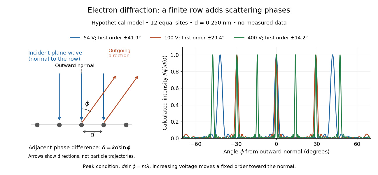
At $100\mathrm{V}$, $\lambda \simeq 0.12264\mathrm{nm}$ and the positive first-order angle is $\arcsin (\lambda /d)\simeq 29.4^{\circ }$. At $400\mathrm{V}$, the wavelength halves and this angle becomes about $14.2^{\circ }$. Increasing $N$ narrows each peak through more selective interference, while increasing momentum brings a fixed-order peak nearer the normal. Unequal site amplitudes, multiple scattering, a three-dimensional crystal lattice structure factor, and finite detector acceptance can change this simple picture; it is an explanatory model with hypothetical inputs.

The Davisson–Germer experiment turned elastic scattering from nickel into evidence for a matter wave. The search became a deliberate wave test in 1926, with diffraction beams found early in 1927. The earlier crystal investigation had begun in 1925; the de Broglie wavelength proposal was already present in the 1924 thesis.^[ref]

A heated tungsten ribbon supplied electrons; gun apertures selected a narrow beam. Two $1\mathrm{mm}$ apertures were $8\mathrm{mm}$ apart; the gun ended $7\mathrm{mm}$ from a nickel crystal cut parallel to its $\{111\}$ planes. An adjustable electric potential difference set the speed. The beam struck normally inside an evacuated, field-free enclosure with target and outer electrodes at one potential. A double-box collector, $11\mathrm{mm}$ from the target with a $1\mathrm{mm}$ entrance, selected directions. A retarding electric potential difference rejected slower electrons; the inner collector fed a sensitive galvanometer. Moving the collector scanned colatitude; rotating the crystal scanned azimuth.^[ref]

The readout was collected electric current, not a photograph of electron paths. Voltage scans held the gun-plate current constant because incident-beam current could not be held constant; the overall current trend therefore needed caution. A strong feature developed at $54\mathrm{V}$ near $50^{\circ }$ colatitude. Surface heating distinguished crystal beams from adsorbed-gas beams; finite apertures and background shifted or broadened apparent peaks.^[ref]

At the bright beam's colatitude, an azimuth scan revealed three companion directions, matching crystal symmetry. The test compared wavelengths inferred from diffraction angles and known crystal spacings with wavelengths inferred from accelerating voltage and momentum; the 1937 lecture displayed this comparison against $U^{-1/2}$. Agreement across beam directions supplied more evidence than one angular peak.^[ref]

The inference is about coherent quantum phases in scattering probabilities. It does not establish a wavy particle trajectory, and a collector-current experiment does not resolve individual detection events. Predicting the full intensity additionally requires the material's scattering amplitude, its surface condition, and instrumental angular acceptance; the de Broglie wavelength alone predicts none of those strengths. The following finite-row electron diffraction model isolates phase addition without attempting to reproduce the nickel measurements.

With signature $(+,-,-,-)$ and $\mathcal{L}=-F_{\mu \nu }{F}^{\mu \nu }/4$, combine a time translation $\alpha {\partial }_0{A}_{\nu }$ with the gauge transformation of parameter $-\alpha A_0$. Its Noether current is $J^{\mu }=-F^{\mu \nu }{F}_{0\nu }-{\delta }_0^{\mu }\mathcal{L}$, the gauge-invariant energy current. The density is $(|\mathbf{E}{|}^2+|\mathbf{B}{|}^2)/2$. On the source-free field equations it differs from the canonical translation current by ${\partial }_{\nu }(A_0{F}^{\mu \nu })$, an antisymmetric superpotential divergence, so total energies agree when the boundary term vanishes.

For signature $(+---)$ in Gaussian electromagnetic units, $T^{ab}=(4\pi {)}^{-1}[-F^a{}_c{F}^{bc}+g^{ab}{F}_{cd}{F}^{cd}/4]$. The Electromagnetic Bianchi identity gives $F^{bc}{\nabla }_b{F}^a{}_c={\nabla }^a(F_{cd}{F}^{cd})/4$, so differentiating the stress tensor proves the displayed identity. Stress conservation implies the source-free Maxwell equations if the matrix $F^a{}_c$ is invertible; otherwise it only forces the field divergence into that matrix's kernel. Conversely source-free Maxwell equations always imply stress conservation.