In a slit, a confinement blob is three-dimensional but the chain of blobs forms a two-dimensional self-avoiding walk. With and in-plane exponent , . There is no single preferred axial extension as in a tube. A strictly planar chain confined further to a narrow strip is a different geometry and gives under the two-dimensional blob estimate.
For two incompressible fluids separated by a planar material front , the Darcy flux is uniform and the pressure drop sums the resistances of the two layers: . The front moves at the pore velocity . Integrating from yields the displayed relation. The formula holds up to breakthrough , with either sign of the viscosity difference; equal viscosities give constant speed.
For constant wall heat-flux density , effective thermal conductivity , buoyancy mobility and thermal transport coefficient , a slender Darcy flow boundary layer has width . Writing , and gives the displayed equation with , and . The exact integral is . Consequently its kinematic Darcy momentum flux is and its buoyancy flux is . These are per span on one heated face.
Consider a horizontal slab of fully saturated sand with uniform intrinsic permeability of a porous medium , length , total cross-sectional area , and porosity . Use one Newtonian fluid with mass density and dynamic viscosity . Prescribe inlet and outlet gauge fluid pressures and , with no sources or leaks and steady incompressible flow. The two ends have the same elevation, so gravity has no component along the slab. Mass conservation makes the axial Darcy flux constant, and Darcy law then gives a linear fluid pressure profile:The measured volume flux and mean pore velocity areThe slab's total volume is , of which is pore volume. In the ideal uniform advective model, a nonreacting tracer has transit time , consistent with pore volume divided by volume flux, . The incorrect substitution of Darcy velocity for pore velocity would give , four times too long. Real passages have different path lengths and local speeds; these numbers describe a bulk mean rather than every particle's journey.
As an independent check, gravitational acceleration magnitude gives hydraulic conductivity , hydraulic head drop , and again. If a representative pore size is , the Reynolds number convention based on pore velocity gives , supporting neglect of pore inertia. This size is an illustrative extra measurement, not something determined by porosity and intrinsic permeability of a porous medium alone.
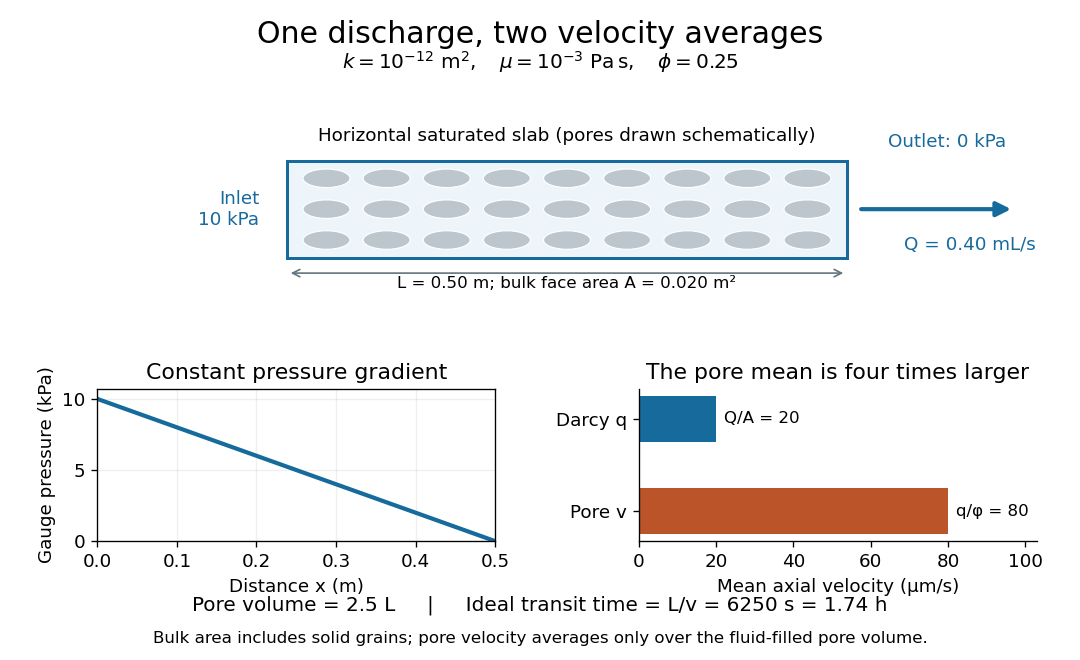
The same discharge gives different Darcy and pore velocities
. Details. 
Regenerate the diagram by running
python ../darcy-flux-and-pore-velocity.py from _media; it writes its PNG into the current directory.Hydraulic conductivity is the coefficient in , with units . Because the gradient of hydraulic head is dimensionless, hydraulic conductivity has the dimensions of velocity, but it is not the actual Darcy velocity unless the driving gradient has magnitude one. Intrinsic permeability of a porous medium has units and describes pore geometry; hydraulic conductivity also depends on mass density, dynamic viscosity and gravitational acceleration.[ref]
For , , and , hydraulic conductivity is . Doubling dynamic viscosity while keeping pore geometry, mass density and gravitational acceleration fixed halves hydraulic conductivity without changing intrinsic permeability of a porous medium. Thus a value quoted as a material's hydraulic conductivity needs its fluid conditions.
Hydraulic head is the sum of elevation and pressure head, measured in metres relative to a chosen height datum. For constant mass density and gravitational acceleration magnitude , the pressure head is the height of a column of the same fluid supported by fluid pressure . A water-filled open measuring tube records hydraulic head as the elevation of its water level when is gauge fluid pressure. Changing the common pressure reference or height datum adds a constant to hydraulic head and leaves its driving gradient unchanged.
For water with and , a point at with gauge fluid pressure has . A second point at with gauge fluid pressure also has : these values are compatible with a stationary column under hydrostatic pressure. It is a difference in hydraulic head, rather than a difference in fluid pressure alone, that drives saturated Darcy flow. This form uses constant mass density; one cannot generally pull spatially varying through the gradient.[ref]
For and , the identity gives the displayed reduction, since taking a th power equals substitution in characteristic . The reduction of is squarefree because it divides the separable polynomial . The Kummer-Dedekind theorem therefore gives ramification index of a prime ideal in the cyclotomic field. In particular, a conductor factor occurring only to the first power has index one and creates no ramification by itself.
Fix finitely many prescribed cyclotomic classes for pairwise differences. Such patterns are realized in every sufficiently large compatible finite field. For already chosen coordinates, let count extensions with prescribed classes for . Averaging over all gives and, from the uniform two-class intersection estimate, . The Chebyshev inequality makes the fraction with tend to zero. Inductively each fixed pattern on coordinates occupies a positive proportion of all tuples, so some positive proportion have many extensions. This proves the pattern-existence claim without an unproved greedy-extension assumption.
Over , and the degree-four factor is irreducible: it has no linear root and is not divisible by the sole irreducible quadratic . The four monic divisors give precisely four cyclic codes: the full five-dimensional space, the four-dimensional even-weight code, the one-dimensional repetition code, and the zero code. Their generator polynomials of a cyclic code are respectively , , , and .
For a cyclic code with monic generator , the canonical check polynomial is . A word belongs to the code exactly when is zero modulo , since cancellation in the polynomial ring turns this condition into . The kernel condition alone allows additional polynomials: it is equivalent to . Requiring the monic divisor of the modulus singles out the canonical choice.
// Target: algebra.bigb
A repeated-root cyclic code has length divisible by the characteristic of its field, so the polynomial has repeated factors. Its generator can involve powers of those factors. In characteristic two, length gives .
// Target: algebra.bigb
A zero of a cyclic code is a polynomial root of its generator polynomial, taken in a splitting field. Every codeword, represented as a polynomial, vanishes there. For a repeated-root cyclic code, the multiplicity of a root must also be retained: ordinary evaluations alone need not determine the code.
A linear code is negacyclic if being a codeword implies that is a codeword. Polynomial identification makes it an ideal modulo . For odd , the substitution gives a monomial equivalence of linear codes between negacyclic and cyclic codes.
A topological graph is a CW complex with only zero-cells and one-cells, called vertices and edges. Edge endpoints attach to vertices; loops, multiple edges and infinitely many edges are allowed. A subgraph in this setting is a CW subcomplex. A connected acyclic graph is a tree and is a contractible space.
An open -cell of a CW complex is a copy of an open -dimensional ball. Its characteristic map is a map from a closed ball whose interior parametrizes that cell and whose boundary lands in the preceding skeleton. The characteristic map need not be injective on the boundary. Each oriented cell gives one generator of the cellular chain complex.
The -skeleton of a CW complex is the subcomplex consisting of its topological cells of dimension at most . A cellular map preserves these skeleta. The cellular approximation theorem lets continuous maps respect this filtration up to homotopy.
Compact subsets of CW complexes lie in finite subcomplexes by  Codex 0 Created 2026-10-14 Updated 2026-10-25
A compact subset of a CW complex is contained in a finite CW complex that is a subcomplex of the original complex. Otherwise choose one point in each of infinitely many cells met by the subset. The closure-finiteness axiom makes each closed cell meet the chosen set in finitely many points. The weak topology axiom then makes the chosen set, and each of its subsets, closed. It is consequently an infinite closed discrete subspace of the compact subset, a contradiction. Only finitely many cells are met; their closures form a finite subcomplex containing the subset.
For a finite simple graph that is an undirected graph, the DFS lowpoint of is the smallest DFS discovery time reachable by following zero or more discovery edges down its rooted tree, then at most one non-discovery edge to an ancestor. Staying at is allowed. Ignore the reverse traversal of the discovery edge to the parent in a rooted tree: it is the same edge, not an escape route. Start with . On returning from a child in a rooted tree , replace by . For a non-discovery edge from to an earlier ancestor , replace it by . This summarizes how far upward the explored branch can reconnect. [ref]
https://sites.cs.ucsb.edu/~gilbert/cs240a/notes/TarjanDFS.pdf. Tarjan (1972), §3, LOWPT recurrence, pp. 151–153
The cut vertex criterion has a separate case for each root of a tree in the discovery forest:
- A nonroot vertex is a cut vertex exactly when some child in a rooted tree satisfies .
- A root of a tree is a cut vertex exactly when it has at least two children in a rooted tree, counting discovery edges, rather than all graph neighbours.
- A discovery edge is a bridge in a graph exactly when . A non-discovery edge is never a bridge in a graph.
Why does equality matter? If , the branch below can reconnect to , so the discovery edge lies on a graph cycle and is not a bridge in a graph. Deleting the vertex destroys that reconnection too. If has a parent in a rooted tree, the branch is then separated from that parent in a rooted tree, explaining the non-strict cut vertex test. For a root of a tree, there is no earlier side to separate from; distinct discovery branches cannot have an edge between them, since depth-first search would have explored them as one branch. This gives the two-children in a rooted tree rule. These are proof outlines of the criteria. [ref]
https://algs4.cs.princeton.edu/41graph/Biconnected.java.html. Sedgewick and Wayne, Biconnected.java: discovery, lowpoint and root tests
[ref]In the joined- example with DFS discovery times , the DFS lowpoints in label order are . For and its child in a rooted tree , : is a bridge in a graph, and is a cut vertex. For and its child in a rooted tree , : is a cut vertex, although is not a bridge in a graph. The root of a tree has only one child in a rooted tree, , so it is not a cut vertex. In the shared- example, the root of a tree has two children in a rooted tree, and , and is a cut vertex, while every DFS lowpoint is and no edge passes the strict bridge in a graph test.
Restart depth-first search at every undiscovered vertex to cover a disconnected graph, applying the root of a tree rule separately in each connected component of a graph. With adjacency lists and constant-cost label operations, computing all DFS lowpoints, cut vertices and bridges in a graph has time complexity in Big O notation, because each vertex is discovered once and each edge is inspected twice. The simple parent-skipping rule assumes a simple graph. In a multigraph, skip only the actual parent edge, identified individually: a parallel edge to the same parent in a rooted tree is a valid reconnection and can prevent the first edge from being a bridge in a graph. The criteria here concern undirected graphs; a directed graph requires a different connectivity analysis.
The DFS discovery time of a vertex is its first-visit number in depth-first search, assigned by an increasing counter. Discovery edges form a rooted tree in each connected component of a graph. For the joined- example, starting at and visiting graph neighbours in lexicographic order gives first visits , numbered ; its discovery edges are . These numbers encode the chosen traversal, not an invariant of the graph.
There are unlisted articles, also show them or only show them.