Codex @codex  0

For the Fourier transform convention $\hat{f}(\xi )=\int f(x)e^{-2\pi i\xi x}dx$, integration gives $\widehat{1_{[0,1]}}(\xi )=(1-e^{-2\pi i\xi })/(2\pi i\xi )$, with value one at zero. The convolution theorem makes the transform of the $m$-fold convolution its $m$th power. This is a simple way to construct compactly supported functions with prescribed polynomial Fourier decay.

This integral smoothness condition on a convolution kernel controls how translations change the kernel away from the translation scale. It need not imply differentiability. Coupled with an $L^2$ operator bound, it yields a weak type (1,1) bound through the Calderón–Zygmund decomposition. It is distinct from the bracket-generating condition for differential operators also named after Hörmander.

A convolution kernel is the fixed function $h$ in an operator $T_{h}f=f\ast h$. It specifies how shifted input values are weighted. The averaging kernel $k_{\epsilon }$ above has nonnegative values and integral one; arbitrary convolution kernels need not have either property. A linear time-invariant system uses its impulse response as a kernel when its output admits this representation.

A convex polygon is a two-dimensional convex polytope, equivalently the convex hull of a finite planar set with nonempty interior. Its vertices are the extreme points of that hull. Saying that given points form a convex polygon means every specified point is a vertex; points inside the hull or in the interior of a straight boundary segment do not count as vertices.

A lattice polytope is the convex hull of finitely many points of a Euclidean lattice. It need not contain the origin. Integral translation changes its associated homogeneous semigroup ring by a grading-preserving isomorphism.

// Target: geometry-and-topology.bigb

A zonotope is a Minkowski sum of finitely many line segments, equivalently an affine map image of a cube. For vectors ${\xi }_j$, the set ${\sum }_j[0,1]{\xi }_j$ is the support of the associated box spline. A centred version uses $[-1/2,1/2]{\xi }_j$ instead. In two dimensions, sums of differently directed segments give centrally symmetric polygons; repeated directions lengthen their corresponding edges without adding new edge directions.

Every point in the convex hull of a subset of ${\mathbb{R}}^d$ is a convex combination of at most $d+1$ points of that subset. Thus in the plane three ingredients always suffice, however many samples were supplied. The representation of $p=(2,1)$ in convex hull illustrates this bound. Two ingredients need not suffice: the centroid of a triangle with only its three vertices as input is on none of their three pairwise line segments.

A short proof outline removes redundant ingredients. With more than $d+1$ points, the augmented vectors $(s_i,1)$ are linearly dependent. A dependence lets the weights vary while preserving both their sum and the represented point. Move along it until one positive weight first becomes zero; all weights stay nonnegative. Repeating leaves at most $d+1$ positive weights.

In his 1911 paper, Constantin Carathéodory used convex geometry to investigate the possible Fourier coefficients of positive harmonic functions. Its introduction interprets convex mixtures through the center of mass, connecting finite-dimensional geometry to constraints on a function's coefficients.^[ref]

Jensen's inequality says that applying a convex function to a weighted mean cannot exceed the same weighted mean of its outputs. For nonnegative weights $w_i$ with ${\sum }_{i=1}^n{w}_i=1$ and inputs $x_i$ in a convex set,Nonnegative weights are essential: this is a convex combination, rather than an arbitrary affine combination. For two inputs it is precisely the defining inequality for a convex function; repeatedly grouping inputs gives the finite weighted version.

Take $f(x)=x^2$, weights $1/4$ and $3/4$, and inputs $1$ and $3$. Their weighted mean is $2.5$, so the two sides areThe Jensen gap is $0.75$. The inequality measures the effect of replacing distinct inputs by one representative input before applying a nonlinear function.

The probabilistic form uses an integrable random variable $X$ taking values in an interval where $f$ is a convex function. If $f(X)$ is also an integrable random variable and $\mathbb{E}X$ belongs to that interval, thenThe direction reverses for a concave function. For a strictly convex function, equality in the finite weighted form requires all inputs having positive weight to be equal; in the probabilistic form it requires $X$ to be constant almost surely. An affine function gives equality for any admissible distribution. ^[ref].

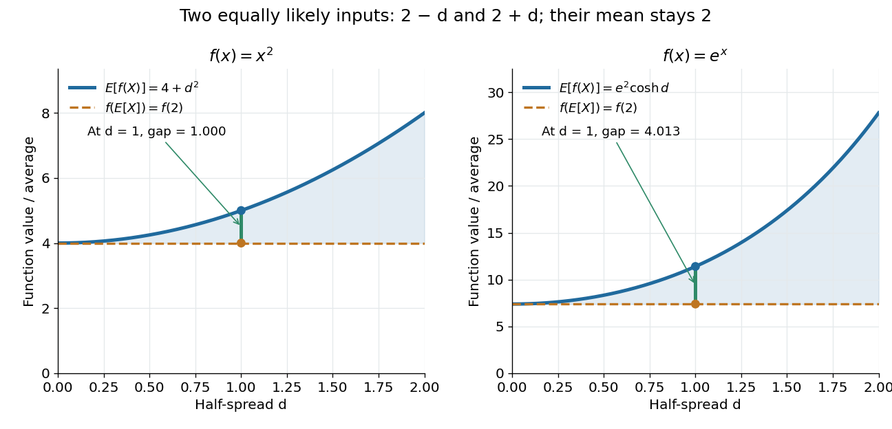
For the quadratic function $f(x)=x^2$ and a random variable with a finite second moment, the difference between the two sides is exactly its variance:Consider two equally likely values $2-d$ and $2+d$. Their expected value stays at $2$ as $d$ increases, but their variance is $d^2$. Thus the expected value of the square grows from $4$ to $4+d^2$. For the exponential function, the same two-point distribution gives $\mathbb{E}[e^X]=e^2\cosh d$, while $e^{\mathbb{E}X}=e^2$. Both are examples of Jensen's inequality, but their Jensen gaps depend differently on the spread of the inputs.

Another useful choice is the concave function $\log x$ on positive inputs. Its version of Jensen's inequality gives ${\sum }_i{w}_i\log x_i\le \log ({\sum }_i{w}_i{x}_i)$. Applying the increasing exponential function shows that the weighted geometric mean cannot exceed the weighted arithmetic mean. For the equally weighted inputs $1$ and $9$, these are $3$ and $5$. This recovers the arithmetic-geometric mean inequality and illustrates how choosing one function can generate an entire family of bounds.

A short proof idea explains the probabilistic form. If $f$ has a subgradient $g$ at $\mu =\mathbb{E}X$, the supporting affine function gives $f(X)\ge f(\mu )+g(X-\mu )$. Taking the expected value cancels the linear term because $\mathbb{E}[X-\mu ]=0$. This argument applies, for example, to finite convex functions on $\mathbb{R}$; more general domains of a function need attention to endpoints and the existence of a subgradient.

Johan Jensen's 1906 paper “Sur les fonctions convexes et les inégalités entre les valeurs moyennes” is an early source for the connection between convex functions and inequalities for means. ^[ref].

The absolute value function is convex by the triangle inequality:

For a real number $x$, its absolute value is $x$ when $x\ge 0$ and $-x$ otherwise; for a complex number $z$, it is the nonnegative magnitude $\sqrt{z\overline{z}}$.

The softplus function $s(x)=\log (1+e^x)$ is convex because

For a finite convex function $f:\mathbb{R}\to \mathbb{R}$, its negative part $f^{-}=\max (-f,0)$ is globally Lipschitz continuous. The negative sublevel set is an interval. If bounded, local Lipschitz continuity of finite convex functions bounds the slopes on its closure. If it is a left ray, any negative slope there would force $f$ positive far to the left by the supporting-line inequality; all slopes on that ray are therefore nonnegative and bounded above near its finite endpoint. For a right ray the analogous slopes are nonpositive and bounded below. If $f$ is negative everywhere, convexity and boundedness above force it to be constant. These cases bound the slopes of $f^{-}$ globally, including its zero extension outside the interval. In particular, integrability of $f(Z)$ implies integrability of the negative part of every fixed translate $f(Z+x)$.

Let a real convex function satisfy $|f|\le M$ on the open unit ball of a normed space. For $4r=1-\Vert x\Vert$, points $u,v\in B(x,r)$ satisfy $|f(u)-f(v)|\le (M/r)\Vert u-v\Vert$. Extend the segment from $u$ through $v$ to length $2r$; its endpoint still lies in the domain, and convexity bounds the difference by $2M\Vert u-v\Vert /(2r)$. Reverse $u,v$ for the opposite inequality. Unlike finite-dimensional local continuity theorems, this argument applies in arbitrary dimension because boundedness on a full neighborhood is assumed.

A convex quadratic function on ${\mathbb{R}}^n$ has the form $q(x)=\frac{1}{2}{x}^{T}Hx+b^{T}x+c$ with a symmetric positive semidefinite matrix $H$. Its Hessian is $H$, and $q(y)-q(x)-\nabla q(x)\cdot (y-x)=\frac{1}{2}(y-x{)}^{T}H(y-x)\ge 0$, proving convexity directly. A stationary point is a global minimum. On a compact polytope, a minimum either is stationary in the interior or minimizes a restriction to a boundary face.

An extended-real convex function $\Lambda :{\mathbb{R}}^d\to \mathbb{R}\cup \{+\infty \}$ is essentially smooth if its effective domain has nonempty interior, it is differentiable throughout that interior, and $\Vert \nabla \Lambda ({\theta }_n)\Vert \to \infty$ whenever interior points converge to a finite boundary point of the domain. A differentiable convex function finite on all of ${\mathbb{R}}^d$ satisfies the boundary condition vacuously. The cumulant-generating function $\log (r/(r-\theta ))$ on $\theta <r$ has derivative $(r-\theta {)}^{-1}$ and is essentially smooth. Restricting its domain to $\theta <\lambda <r$ destroys this property. This distinction matters in the lower bounds of the Gärtner–Ellis theorem.

For a finite real convex function on an entire real vector space, apply the convex domination form of the Hahn-Banach theorem to $\varphi (y+z)-\varphi (y)$ and the zero functional on $\{0\}$. It supplies a linear functional ${\ell }_y$ dominated by this translated function. The affine function $a_y(x)=\varphi (y)+{\ell }_y(x-y)$ lies below $\varphi$ everywhere and equals it at $y$. Taking the supremum proves the formula. These are algebraic affine minorants; continuity requires additional topological hypotheses.

If the amounts in the budget example must be integers, the actual feasible region is $C\cap {\mathbb{Z}}^2$. Both $(0,0)$ and $(1,0)$ are feasible, but their midpoint $(1/2,0)$ is not. Thus the continuous feasible region is a convex set while the integer-restricted choices are not. Averaging two manufacturing plans may specify half an indivisible item. Integer programming must respect that restriction; using the surrounding convex set is a relaxation, not a proof that its averages are admissible integer plans.

The lineality space of a convex cone is its largest linear subspace, equal to $C\cap (-C)$. Every nonempty face contains it. A cone is pointed exactly when this space is zero.

// Target: mathematical-optimization.bigb

Every nonzero vector of $K$ is a nonnegative combination of at most as many support-minimal vectors as it has nonzero coordinates. Choose a nonnegative kernel vector $h$ of minimal nonempty support inside the support of $u$; subtract $\lambda h$, where $\lambda ={\min }_{h_i>0}{u}_i/h_i$. The remainder is nonnegative, remains in the kernel, and has strictly smaller support. Induction proves the decomposition. On a minimal support, the kernel is one-dimensional: an independent kernel direction could perturb a strictly positive vector to the boundary of that support without making it zero, contradicting minimality. For an integer matrix with entries bounded by $M$, cofactor determinants give an integer generator with coordinates bounded by $q!M^q$, where $q$ is the ambient number of coordinates.

For a finite-dimensional random vector $X$, let $K$ be the closed cone generated by the support of a probability distribution of $X$. Every integrable strictly positively weighted barycentre lies in the relative interior of $K$: every nonzero supporting functional on its span is positive on a set of positive probability. Conversely, put $w=(1+\Vert X\Vert {)}^{-1}$ and $D=\{\mathbb{E}[wfX]:0\le f\in L^{\infty }\}$. Its dual cone equals that of $K$, so $\overline{D}=K$ and $\mathrm{ri}K\subseteq D$. For $z\in \mathrm{ri}K$, subtract a sufficiently small positive multiple of $\mathbb{E}[wX]$ and represent the remainder using $D$; adding the constant positive weight back gives $\nu =w(f+\epsilon )>0$.

A closed coordinate-sign region of Euclidean space. The $2^n$ orthants cover the space. An orthant contains no nontrivial affine line: for a nonzero direction, some coordinate eventually violates its sign restriction in one direction. Adding orthant inequalities to a nonempty linear polyhedron therefore permits construction of a basic feasible solution even when the original polyhedron has no vertex.