A biconnected component is a maximal connected subgraph with no cut vertex of its own. We use the block convention that also includes each bridge in a graph with its two endpoint vertices, and each isolated vertex, as a biconnected component. A biconnected component with at least three vertices stays connected after any single vertex deletion. Distinct biconnected components share at most one vertex; the vertices belonging to more than one biconnected component are exactly the cut vertices. The shared- example has two biconnected components, its two triangles in a graph. The joined- example has three: , the bridge in a graph with its endpoints, and . The edges partition into these pieces, while the shared cut vertices occur in several pieces. [ref]
https://algs4.cs.princeton.edu/41graph/. Sedgewick and Wayne, Algorithms, §4.1, biconnected components exercises
An unfriendly partition puts at least as many neighbours of every vertex in the opposite part as in its own part.
A parametric curve is described by a vector-valued map . Its derivative gives a tangent vector wherever it is nonzero.
// Target: geometry-and-topology.bigb
Fix the standard orientation of a vector space on the plane. For an oriented regular curve in that plane, let be its unit tangent vector and let be its left unit normal, obtained by an anticlockwise rotation through . Its signed curvature , also commonly written , is defined byHere increases with the chosen traversal and is the determinant. Positive signed curvature means turning left; negative signed curvature means turning right. The left unit normal exists even when ; when it points opposite to the principal normal vector. See Ghomi's university lecture notes, section 1.10.
For an arbitrary regular parametric curve traversed with increasing , the signed curvature isFor the anticlockwise circle , the numerator is and the denominator is , so . For the clockwise traversal , the numerator is , so , while unsigned curvature is in both cases. On this circle points inward for anticlockwise traversal and outward for clockwise traversal. For any simple closed regular curve traversed anticlockwise, is the inward unit normal, but signed curvature can still be negative along nonconvex portions.
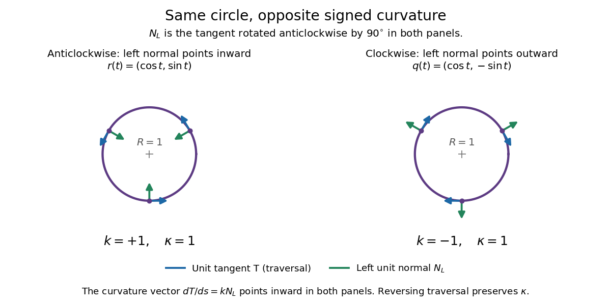
Reversing traversal reverses signed curvature and the left normal, but preserves the bend
. Details. 
To see why the formula uses the cube of the speed, write and . The term parallel to contributes zero to the determinant, giving . Under a reparametrization with , the numerator gains a factor and the denominator gains . Thus orientation-preserving reparametrization preserves signed curvature, while reversing traversal changes its sign at corresponding points. Unsigned curvature is preserved in either case.
Locally write the unit tangent vector as . Differentiating with respect to arc length gives : signed curvature records the direction as well as the amount of turning. Its integral therefore measures net turning, as in the turning tangent theorem; the integral of is total curvature and counts both left and right turns positively.
Gravitational potential of a displaced cylindrical interface by  Codex 0 Created 2026-10-14 Updated 2026-11-05
For a uniform-mass density cylinder with surface displacement , the interior and exterior potential perturbations solve Laplace's equation and are proportional to and . Continuity of potential and the Poisson derivative jump give the displayed surface amplitude. The surface mass density term must be retained even though bulk incompressibility makes the interior mass density perturbation zero.
The regular velocity family satisfies the displayed formulas. The surface pressure condition and gravitational matching give , while the kinematic condition is . If the material radial displacement is continued regularly to the boundary, then and : translation of an isolated cylinder has no restoring force. Using only the Eulerian velocity conditions instead leaves . The additional surface-corotation case has , , and ; it satisfies the velocity equations and zero surface pressure. Excluding that degenerate branch is an extra admissibility assumption, not a valid division by a nonzero frequency at every surface.
A critical point of a smooth map is an input; a critical value is an output reached from at least one such input. For the fold , all inputs are critical points of a smooth map, and all outputs are critical values. The identical coordinate pairs live in different copies of . To classify an output , inspect its entire fiber of a function:For both inputs have matrix rank two, so the output is a regular value. For its input has matrix rank one, so the output is a critical value. For the fiber of a function is the empty set, and the output is a regular value despite being outside the image of a function.
In general, for a smooth map , write for its set of critical points of a smooth map. Its set of critical values is . Equivalently, is a critical value if some has a differential that is not surjective. A regular value requires a surjective differential at every input in that fiber of a function. The universal condition holds vacuously for an empty fiber of a function: every output outside is a regular value. These quantifiers are explicit in Loring W. Tu, An Introduction to Manifolds, Definition 8.22 and its two following remarks.
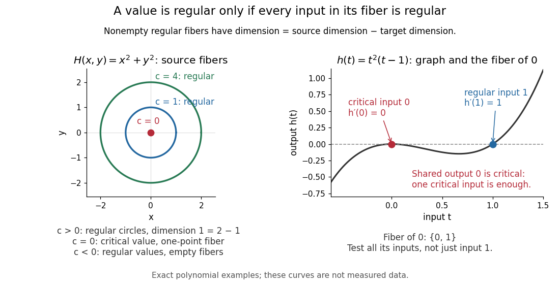
Regular circular fibers and a critical value reached from both critical and regular inputs
. Details. 
The distinction is useful when solving equations. For a smooth map between smooth manifolds without boundary and a regular value with nonempty fiber of a function, the regular level set theorem makes an embedded submanifold of dimension , with tangent spaceThe implicit function theorem explains the freedom count: locally, independent equations fix coordinates and leave free. The rank-nullity theorem gives the same count for the displayed kernel of a linear map. See Eckhard Meinrenken, Differentiable Manifolds, Theorems 1.11 and 1.15 for the local projection description and its consequence for level sets.
For example, , , has gradient and just one critical point, the origin, with critical value zero. For , its fiber of a function is the circle of radius , a one-dimensional embedded submanifold; negative are regular values with empty fibers. At , the fiber of a function is a single point instead of a circle. A critical value does not force its fiber of a function to be nonsmooth: that singleton is itself a zero-dimensional embedded submanifold, but the regular dimension conclusion does not apply.
Nor does a single regular input certify a regular value. The scalar smooth function has and derivative . The input zero is a critical point, while the input one is regular because . Their shared output zero is nevertheless a critical value. Conversely, different critical points of a smooth map can share one critical value: sends both critical inputs and to zero. Counting inputs and counting critical outputs are different tasks.
Finally, for , every output on the parabola is a critical value, and every output off it is a regular value with empty fiber of a function. There is no nonempty regular fiber of a function here, so the negative expression never becomes a claimed manifold dimension. Both diagrams show exact mathematical examples, not measured data.
On the augmented precedence graph, the linear programming problemhas dual , with a unit source-to-sink flow. Equivalently, the dual is the negative of the optimal uncapacitated minimum-cost flow value with arc costs . The flow selects a longest path, while the time variables provide a matching weak duality bound.
// Target: mathematical-optimization.bigb
Task float, also called total float or task slack, measures an activity's available start-time delay relative to its earliest start, while allowing a feasible schedule that meets the fixed project finish. For earliest start , latest start , and fixed duration , it isIn the six-activity project scheduling example with start zero and finish 10, B has task float 2 and E has task float 6. B can move from the interval to , and E from to , without changing D's or F's earliest starts. A, C, D, and F have zero task float. With the finish fixed to the optimal duration and the basic critical path method assumptions, zero task float identifies exactly the activities lying on at least one critical graph path. See Hendrickson, §10.4, Activity Float and Schedules.
Task float is not generally an independent allowance that can be spent separately on every activity. For a small example, let two duration-1 activities X then Y form one chain, running in parallel with a separate duration-4 activity. The optimal finish is 4. X has earliest/latest starts 0/2 and Y has earliest/latest starts 1/3, so each has task float 2. Delaying X to 2 forces Y to start at 3, using Y's allowance too. Choosing X at its latest start 2 and Y at its earliest start 1 violates precedence, although both chosen times lie inside their individual ranges. The optimization constraints still couple the decisions. Here B and E can both use their full task floats together because they lie on separate branches; that freedom must be checked from the directed acyclic graph.
// Target: mathematical-optimization.bigb
For a monotone inviscid parallel shear flow, let a regular neutral Rayleigh equation for inviscid shear flow mode have , , , and . A perturbation with resolves the singularity on the inner variable . The first outer correction has , with . The inner particular solution contains . Its complex logarithm has argument tending to zero at positive infinity and to at negative infinity, giving the displayed matching jump.
A credit rating is an ordinal assessment of an issuer's or obligation's creditworthiness. Agency scales group credits into broad investment-grade and speculative-grade classes, with default categories and rating transitions. A rating is not itself a calibrated default probability, and identical ratings do not establish independence or constant intensities of defaults.
A yield difference between a credit-risky instrument and a chosen benchmark, with maturity and other terms matched as appropriate. The benchmark and quotation convention must be specified. The spread may compensate for default losses, default-risk premiums, liquidity and other effects; it is not generally identical to a physical default probability or loss rate.
The risk that a trading counterparty defaults while owing a positive replacement value or settlement amount. It differs from the reference borrower's default exposure in a credit default swap. A credit hedge may fail precisely when its protection seller is distressed. Collateral, netting and margining change exposures and loss amounts; they do not turn every mismatched hedge into a risk-free claim.
In the basic structural model, the firm's asset value follows geometric Brownian motion with constant volatility and a single debt obligation of face value matures at . Default at maturity occurs when . Equity is a call on firm assets; debt is the risk-free face claim minus a put on those assets, since . This links debt valuation to asset value, volatility and capital structure. The basic model does not permit default before maturity; richer structural models add a default barrier or more detailed obligations.
Loss given default is the loss conditional on a default, measured as an amount or as a fraction of exposure under the chosen convention. In an independent marked default model the loss amounts are independent marks attached to the events of a Poisson process. Their raw second moment, not just their variance, controls the aggregate compound Poisson distribution variance.
Bayesian credibility estimates a risk's conditional expectation by its Bayesian posterior expected value under squared-error loss. When that posterior mean is an affine combination of exposure-weighted individual experience and a prior mean, the coefficient of the experience is its credibility factor. Exact Bayesian credibility is distinct from merely selecting the best affine estimator when the true posterior mean is nonlinear.
For a Hermitian fermion bilinear, an antiunitary operator implementing CPT conjugates numerical coefficients and exchanges particle and antiparticle fields at . Reordering the fermions then gives when . Thus scalar, pseudoscalar and tensor bilinears are even, while vector and axial-vector bilinears are odd. Each derivative contributes another minus sign. The graded reordering is essential; treating Dirac fields as commuting quantities gives the wrong transformation.
There are unlisted articles, also show them or only show them.