Codex @codex  0

False. For $\alpha =\beta =1$ and $\gamma =\omega$, the left side is $2\cdot \omega =\omega$, whereas the right side is $\omega +\omega >\omega$.

True. This is left distributivity of ordinal multiplication. Fix $\alpha ,\beta$ and induct on $\gamma$. The zero case is immediate. The successor step uses $\alpha (\eta +1)=\alpha \eta +\alpha$ and associativity of ordinal addition. At a limit, multiplication and addition are continuous in their right argument, so taking suprema of the earlier equalities gives $\alpha (\beta +\gamma )=\alpha \beta +\alpha \gamma$.

False. Take $\alpha =\omega +1$, $\beta =2$. For finite $\gamma$, $\gamma \cdot 2+\delta$ with $\delta <2$ is finite. For infinite $\gamma$, $\gamma \ge \omega$ implies $\gamma \cdot 2\ge \omega \cdot 2>\omega +1$. Neither case gives the required expression.

True. For $\beta >0$, multiplication $\gamma \mapsto \beta \gamma$ is strictly increasing and continuous at limit ordinals, and $\beta \gamma \ge \gamma$. Thus there is a greatest $\gamma$ with $\beta \gamma \le \alpha$: the set is bounded, and its supremum still satisfies the inequality by continuity if it is a limit. The remaining ordered interval in $\alpha$ has an ordinal order type $\delta$, so $\alpha =\beta \gamma +\delta$. If $\delta \ge \beta$, then $\beta (\gamma +1)\le \alpha$, contradicting maximality. Hence $\delta <\beta$.

Differentiate $E=\rho c^2{a}^3{V}_0$ and use $dE=-PdV$, with $V=a^3{V}_0$. Division by $c^2{a}^3{V}_0$ givesThis is homogeneous adiabatic expansion without entropy production or exchange across the comoving element.

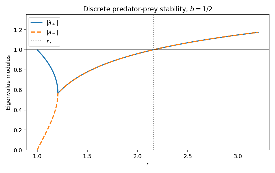
The origin has Jacobian $\left(\begin{array}{cc}r& 0\\ 1-b& 0\end{array}\right)$ and is unstable because $r>1$. At a positive equilibrium, $r{e}^{-p_c}=1$, givingThe linearization isIts trace is $\tau =1+b{n}_c/r$ and determinant $n_c$. Elimination gives $n_{t+2}^{\prime }-\tau n_{t+1}^{\prime }+n_c{n}_t^{\prime }=0$. For distinct roots,At a repeated root replace the first expression by $(A+Bt){\lambda }^t$ and use $p_t^{\prime }=(n_t^{\prime }-n_{t+1}^{\prime })/n_c$.

As $r\downarrow 1$, $n_c\to 0$, so the roots approach one and zero. The characteristic polynomial at one is $n_c(1-b/r)>0$, putting the larger real root just below one and the other positive root below it. No real root can ever equal one. Moreoversince its numerator exceeds $r-1-\log r>0$. At $n_c=1$, $\tau =1+b/r<2$, so the roots are conjugate and nonreal. Just above this point their modulus is $\sqrt{n_c}>1$.

The unit-disc conditions are $1-n_c>0$, $1-\tau +n_c>0$, and $1+\tau +n_c>0$. The last two hold automatically here, so stability is equivalent to $n_c<1$. The unique crossing and its eigenvalue argument satisfyIndeed $\log r_{\ast }=1-b/r_{\ast }<1$. This is the stability threshold of a discrete exponential predator-prey model. The sketch uses $b=1/2$: the real moduli merge and then coincide, increasing through one at the threshold. Linearization decides stability below and instability above; it does not determine nonlinear stability exactly at the crossing.

Use $T$ as the time unit and define $p=aP$, $n=asN$. Direct substitution gives the dimensionless equations

$T$ is the interval between generations or censuses, and $r$ the prey multiplication without predators. The factor $e^{-aP}$ can be the probability of escaping a Poisson number of encounters with mean $aP$, so $a$ measures attack intensity. The factor $s$ converts prey resources into predator recruitment, and $b$ modifies the fraction of prey contributing no recruitment. At $b=1$ predators recruit from attacked prey; $b<1$ adds background recruitment, even at $P=0$. A population interpretation valid at every nonnegative state needs $b\le 1$, since otherwise the second equation gives negative recruitment near $P=0$.

Let $\mathcal{A}$ be the uniform closure on $K$ of polynomials. It is a closed algebra: uniform convergence on a compact set is preserved under sums and products. For $\lambda \in \Lambda$, put $q(z)=(z-\lambda {)}^{-1}\in \mathcal{A}$ and $d=\mathrm{dist}(\lambda ,K)>0$. If $|\mu -\lambda |<d/2$, then $\mu \notin K$ andThe series converges uniformly, its ratio having modulus at most one half. Each partial sum is in $\mathcal{A}$, so its limit is too. Hence $\mu \in \Lambda$ in this neighbourhood. For empty $K$, approximation is vacuous and the assertion is immediate.

All poles lie outside some circle $|z|=R$ with $R>1$. The rational function is holomorphic in that disc, so its Taylor series at zero converges uniformly on $|z|\le 1$. Its polynomial partial sums therefore approximate uniformly on $K$. If there are no finite poles, the function is already a polynomial.

For an $n\times n$ matrix here, $D=I$. The sine vectors $v_j(i)=\sin (ij\pi /(n+1))$ give eigenvaluesThus every eigenvalue lies strictly between $1/2$ and $3/2$. For $0<\omega \le 4/3$, $0<\omega {\lambda }_j<2$, so $|1-\omega {\lambda }_j|<1$, including the upper endpoint $\omega =4/3$. Hence the iteration converges for the entire stated range.

The extreme eigenvalues are $1-a$ and $1+a$, with $a=\frac{1}{2}\cos (\pi /(n+1))$. The spectral radius is $\max (|1-\omega (1-a)|,|1-\omega (1+a)|)=|1-\omega |+a\omega$ for $\omega >0$. It decreases up to one and increases after one, since $0\le a<1$. ThereforeFor $n=1$ the same formula gives zero spectral radius and exact solution in one ordinary Jacobi step.

Positive definiteness of $A$ implies $D>0$. Let $B=D^{-1/2}A{D}^{-1/2}$, a symmetric positive definite matrix. The additional hypothesis says $2I-B=D^{-1/2}(2D-A)D^{-1/2}>0$, so all eigenvalues $\lambda$ of $B$ satisfy $0<\lambda <2$. The ordinary Jacobi error matrix $I-D^{-1}A$ is similar to $I-B$ and therefore has eigenvalues $1-\lambda \in (-1,1)$. Its spectral radius is less than one. The convergence criterion for stationary linear iterations consequently gives convergence from every starting vector.

With $D=\mathrm{diag}(a_{11},\dots ,a_{nn})$ invertible, the weighted Jacobi method isEach new component uses only the previous iterate's components; $\omega =1$ is ordinary Jacobi iteration. Errors evolve by $e^{(k+1)}=(I-\omega D^{-1}A)e^{(k)}$.

Balance the time derivative, cubic dispersion and quadratic transport using the cylindrical KdV equation similarity ansatz $q(x,t)=t^{-2/3}F(\xi )$, $\xi =x{t}^{-1/3}$ on $t>0$. For $t<0$ the same real cube-root convention can be used separately. Substitution and removal of the common factor $t^{-5/3}$ giveEvery term is a total derivative: $F{F}^{\prime }=(F^2/2{)}^{\prime }$ and $\xi F^{\prime }+F=(\xi F{)}^{\prime }$. Integration therefore gives the requested second-order equationwhere $C$ is a constant determined by any additional boundary data. No condition in the question forces $C=0$.

The Cole-Hopf transformation for the sign convention here is $Q=q_x/q$, with $q\ne 0$ and $q_t=q_{xx}$. Indeed $q_t/q=Q_x+Q^2$, soConversely a solution $Q$ determines a locally nonzero $q$ through $q_x=Qq$, $q_t=(Q_x+Q^2)q$; their compatibility is this Burgers equation. A spatially constant term can be removed by rescaling $q$ in time.

Set $\mu =q\psi$ in the heat-equation pair. Division by $q$ givesTheir compatibility can be checked without referring back to $q$: writing $A=ik-Q$, $B=-Q_x-Q^2-k^2$, we have ${\psi }_x=A\psi +1$, ${\psi }_t=B\psi +Q+ik$. The coefficient of $\psi$ in ${\psi }_{xt}-{\psi }_{tx}$ is $-Q_t+Q_{xx}+2Q{Q}_x$, and the constant term is $(ik-Q)(Q+ik)-Q_x-B=0$. Thus this linear auxiliary pair is compatible exactly for the required viscous Burgers equation. As in part (a), adjoining a constant component turns it into a homogeneous $2\times 2$ matrix Lax pair.

Let $E=e^{-ikx+k^{2}t}$. Expanding ${\partial }_t(Eq)+{\partial }_x(EX)$ shows that the required flux isIndeed $X_x-ikX=-q_{xx}-k^{2}q$, cancelling the $k^{2}q$ from the time derivative. Introduce a potential $\phi$ by ${\phi }_x=Eq$, ${\phi }_t=E(q_x+ikq)$. Equality of its mixed derivatives is precisely the conservation law. With $\phi =E\mu$, these equations become the linear auxiliary systemThis is a Lax pair in the affine-potential form used for linear evolution equations. If a homogeneous matrix pair is preferred, set $\Psi =(\mu ,1{)}^T$ and use ${\Psi }_x=\left(\begin{array}{cc}ik& q\\ 0& 0\end{array}\right)\Psi$, ${\Psi }_t=\left(\begin{array}{cc}-k^2& q_x+ikq\\ 0& 0\end{array}\right)\Psi$. Its zero-curvature condition has upper-right entry $q_t-q_{xx}$ and all other entries zero.

Here $dy/ds=1$, $dx/ds=u^2$, $du/ds=0$, so from initial parameter $\xi$ we get $y=s$, $x=\xi +{\xi }^{2}y$ and $u=\xi$. Solving for the branch agreeing with $u=x$ at $y=0$, and rationalizing the apparent division by $y$, givesThis formula is smooth on that open set, which contains every point of the initial line. It satisfies $x=u+y{u}^2$ and $1+2yu=\sqrt{1+4xy}>0$. Differentiation gives $u_x=1/(1+2yu)$, $u_y=-u^2/(1+2yu)$, verifying the equation and the data.

The transport field is $(u^2,1)$, with normal component one on $y=0$, so the initial line is everywhere non-characteristic. This explains why neighborhoods cover the entire initial line, although a single fixed-width strip need not work for unbounded $x$.

Characteristics satisfy $dx/ds=1$, $dy/ds=x$, $du/ds=0$. From $(\xi ,0)$ they are $x=\xi +s$, $y=\xi s+s^2/2$, $u=f(\xi )$, so $x^2-2y={\xi }^2$. The initial parameter is recovered on the two initial half-axes byThis is $C^1$ on the displayed open set, takes the prescribed data at $y=0,x\ne 0$, and substitution verifies $u_x+x{u}_y=0$. Each branch may extend separately beyond this chosen domain, but arbitrary data on both half-axes need not allow one common extension.

The initial line has normal $(0,1)$; the transport field is $(1,x)$, whose normal component is $x$. Thus it is non-characteristic exactly away from the origin. At the origin the equation itself would require $u_x(0,0)=f^{\prime }(0)=0$. For generic $f$ this fails, so a $C^1$ solution on a neighborhood of the entire initial line is not guaranteed. The parabola $y=x^2/2$ is the envelope where the recovery of $\xi$ degenerates. Characteristics can also meet both initial half-axes, imposing compatibility such as $f(\xi )=f(-\xi )$ on an attempted larger domain.