The variance measures the mean squared distance of a random variable from its expected value. For a real square-integrable random variable ,The square prevents positive and negative deviations from cancelling. It also gives the variance squared units: if measures a length in metres, its variance has units of square metres. Its nonnegative square root is the standard deviation, which has the same units as .
For example, let take , and with equal probabilities. Its expected value is zero, but its variance is , and its standard deviation is . The constant random variable zero has the same expected value and zero variance: a mean alone does not describe the spread. The variance is zero exactly when almost surely.
The variance is useful because squared deviations interact neatly with linear combinations. The covariance supplies the cross terms when combining different random variables, and a covariance matrix organizes those terms for many variables. The characterization of variance as the minimum mean squared error of a constant also explains why the expected value is the best constant prediction under squared error.
For transmission through scale heights, a useful estimate isSmall host stars, low gravity, high temperature, and low mean molecular mass make atmospheric features larger.
Atmospheric escape removes gas from a planet through thermal motion, hydrodynamic outflow, photochemistry, and interactions with stellar radiation and plasma.
An exoplanet emission spectrum is the wavelength-dependent thermal radiation emerging from the planet. Vertical temperature gradients turn opacity differences into absorption or emission features.
An exoplanet transmission spectrum measures the wavelength-dependent area blocked as starlight passes tangentially through the atmosphere during transit.
An irradiated planetary atmosphere receives stellar energy from above while internal heat emerges from below. Their competition creates radiative, convective, and sometimes thermally inverted regions.
For oscillators of frequencies and , the perturbationpreserves . On the energy- basis , it is the matrixso the symmetric and antisymmetric combinations are exact eigenstates with shifts .
Let be a finite undirected multigraph, allowing self-loops and distinct parallel edges, with . Thenwhere is the edge support of a graph, and vertex degrees count each self-loop twice. There is no lower bound of three on the number of vertices. If , the zero-length convention gives an Euler circuit exactly when .[ref]
The two requirements are independent: two separate vertices, each carrying a self-loop, have even vertex degrees but disconnected edge support of a graph, so no Euler circuit can cover both edges.
Necessity follows because a single trail cannot cover edges in different connected components of a graph, while a closed trail pairs all arriving and departing incidences, including those at its starting vertex. For sufficiency, extend a trail using unused edges until no extension is possible. Even vertex degree parity prevents it from stopping anywhere except its starting vertex: a different stopping vertex would have an odd number of used incidences and hence at least one unused incidence. The result is a closed trail.
If unused edges remain, connectivity of the edge support of a graph supplies a vertex on the current closed trail with an unused incident edge. Removing a closed trail leaves even unused vertex degrees, so the same argument constructs another closed trail from that vertex. Splice it into the existing record. The two trails use disjoint edge identities, so the splice repeats no edge. Each splice uses more edges; finiteness ensures termination with an Euler circuit. This is the constructive idea of Hierholzer's algorithm.
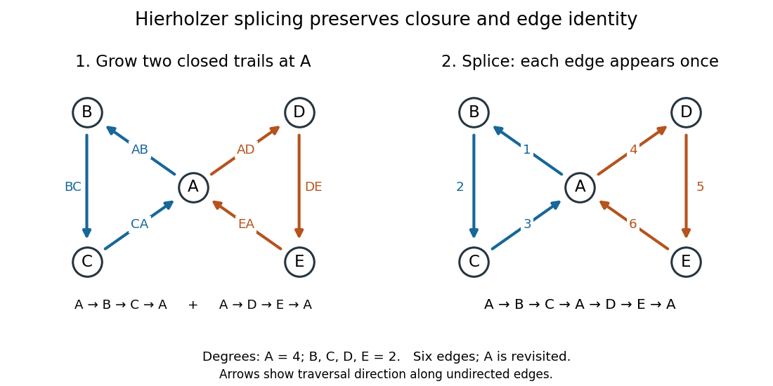
Hierholzer's algorithm inserts one closed trail into another at their shared vertex, using each of six edges exactly once
. Details. 
In the drawing, arrows indicate the chosen traversal direction along undirected edges. The first closed trail uses and the second uses . Insert the second at the final occurrence of in , giving . A reader can check consecutive endpoints, closure, and the six distinct edges directly. With multigraphs, perform the same check on edge identities, since endpoint pairs alone cannot distinguish parallel edges.
For a rigid body with three distinct positive principal moments of inertia and zero external torque about its centre of mass, steady rotation about the first or third principal axis is Lyapunov stable in angular velocity, while rotation about the intermediate principal axis is unstable. Here steady rotation means in the principal body frame, with constant . A small sideways perturbation remains small about the extreme principal moments of inertia, but generically grows about the intermediate one. Stable does not mean that the wobble decays: without damping, there is no asymptotic stability. Coincident principal moments of inertia and a stationary body are excluded.[ref]
3. The Motion of Rigid Bodies. Classical Dynamics by David Tong, §3.4.3, The Asymmetric Top: Stability, printed pp. 57–58, equations (3.40)–(3.45)
No external torque is needed for a body to tumble. Conservation of angular momentum fixes in the fixed space frame, but the body can turn relative to , so its angular velocity components in the principal body frame change. The torque-free rigid-body invariants constrain this motion. A supported gyroscope with gravitational torque has different governing assumptions.
Coplanarity in a torque-free axisymmetric rigid body by  Codex 0 Created 2026-09-24 Updated 2026-09-24
Codex 0 Created 2026-09-24 Updated 2026-09-24For principal moments and symmetry-axis unit vector , angular momentum and angular velocity obeyThus , , and the symmetry axis are coplanar at every instant.
The Euler equations for a torque-free rigid body conserve rotational kinetic energy and squared angular momentum,Their common level sets are the intersection of two ellipsoids in angular-velocity space.
Thermal fluctuations smooth the zero-temperature pitchfork in filament buckling: the mean compression remains analytic and nonzero below the mechanical threshold, with rounding controlled by .
For a fixed point a distance from the centre of mass and inclination measured from the upward vertical,The spin and precession angles are cyclic.
There are unlisted articles, also show them or only show them.