
The Standard Model Higgs field is a complex doublet of hypercharge . Its nonzero vacuum expectation value triggers the Higgs mechanism.
The electromagnetic field tensor isIt packages the electric and magnetic fields into an antisymmetric rank-two Lorentz tensor and transforms as
An electromagnetic multipole expansion expresses the potentials or fields of a localized source as successively smaller monopole, dipole, quadrupole, and higher moments in the ratio of source size to observation distance.
An equipotential is a level set of the electric potential. The electric field is normal to every smooth equipotential.
An electric quadrupole is a charge distribution whose total charge and electric dipole moment vanish while its second charge moment does not. Its potential decays as .
The even, spherically symmetric hydrogen atom ground state has no permanent electric dipole, so a uniform electric field gives no first-order energy shift. The electric-dipole selection rules for hydrogen allow odd-parity excited states to mix in at second order, yielding a negative shift quadratic in the field.
A finite electric dipole consists of equal and opposite electric charges separated by a nonzero displacement. It has charge neutrality but a nonzero electric dipole moment . An ideal point electric dipole is the mathematical limit with fixed, so must increase as . Shrinking the separation while holding fixed instead makes the electric dipole moment vanish. The ideal electric dipole describes an exterior electric field; it does not reproduce the two near-charge singularities or the internal structure of a molecule. [ref]
https://farside.ph.utexas.edu/teaching/jk1/lectures/node20.html. Richard Fitzpatrick, Electric Dipoles: the fixed-moment point limit
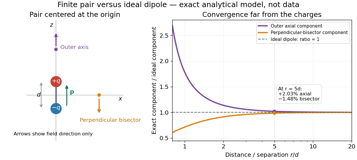
.Place the pair's midpoint at the origin and write , where is vacuum permittivity. By superposition principle and Coulomb's law, its exact electric potential away from the two point charges isFor , retain the first nonzero term of a Taylor series. The electric potential and its negative gradient becomeHere and the products in parentheses are dot products. These are exact exterior formulas for the ideal electric dipole and distant approximations for a finite pair. The electric field on the outer axis points along with magnitude ; on the perpendicular bisector it points opposite with magnitude . This directional structure is what a scalar total electric charge misses. [ref]
https://www.feynmanlectures.caltech.edu/II_06.html#Ch6-S2. Feynman, Leighton and Sands, II.6.2: exact pair potential and dipole expansion
.In a prescribed uniform external electric field , a rigid pair has opposite forces . Its net force is zero, but summing their moments about the midpoint gives the torqueThe cross product makes the torque perpendicular to both the electric dipole moment and the external electric field. If is the angle from to in their plane, the signed turning torque is . It tends to reduce a small positive . [ref]
https://openstax.org/books/university-physics-volume-2/pages/5-7-electric-dipoles. Ling, Moebs and Sanny, University Physics 2, 5.7: forces and torque on a dipole
.The external interaction potential energy, with zero chosen at , isParallel alignment minimizes this potential energy; antiparallel alignment maximizes it even though the torque is zero in both positions. This omits the pair's constant internal binding potential energy and assumes a fixed permanent electric dipole moment. [ref].
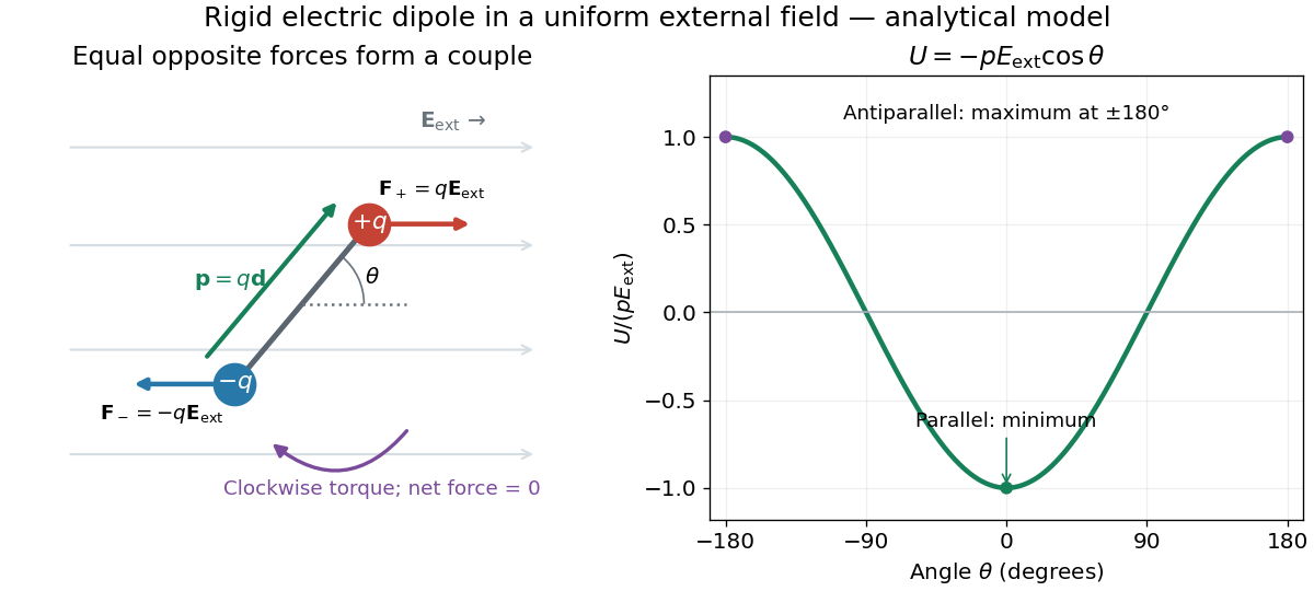

A nonuniform external electric field can exert a net force on a neutral electric dipole. Before taking the small-pair approximation, the exact external force is , where is the midpoint. A first-order Taylor series gives, for a fixed electric dipole moment and an external electric field varying slowly across ,in electrostatics. The last equality uses the vanishing curl of the external electric field, with held fixed while differentiating. Thus uniform external electric fields turn a misaligned electric dipole, whereas gradients can also move its midpoint. For example, the local source-free electric field gives , so reversing the electric dipole moment reverses the net force. This stipulated local model has zero divergence and zero curl.
A motivating experiment is Filsinger and colleagues' study of electrostatic deflection of polar molecules. Benzonitrile () in helium expanded from a pulsed valve into vacuum; two 1-mm skimmers narrowed the beam before a 15-cm deflector. A grounded trough and a high-voltage rod produced a vertical electric field gradient. Scanning a focused laser vertically downstream and recording benzonitrile ions from photoionization measured the beam's relative density. With voltage off, the profile spanned about 2 mm; applying voltage shifted and broadened it upwards. At 10 kV, many molecules lay outside the original profile. [ref]
https://pure.mpg.de/pubman/item/item_736019_2/component/file_736018/433451%28filsinger%29.pdf. Filsinger et al., Quantum state selection, alignment, and orientation of large molecules using static electric and laser fields, sections II and III A, figure 3
.Interpretation uses a quantum state's Stark effect energy : gives . States whose energy falls with increasing electric field seek stronger fields. The voltage-off profile controls the mechanical aperture. Inferring state populations needs calculated trajectories, speed distributions and a rotational temperature model; profile displacement alone does not measure a permanent electric dipole moment uniquely. This is an electric Stark effect experiment, with photoionization occurring after deflection. [ref]
https://pure.mpg.de/pubman/item/item_736019_2/component/file_736018/433451%28filsinger%29.pdf. Filsinger et al., section III A: Stark slopes, trajectory modelling and state selection
.For the symmetric finite pair, the first omitted electric multipole expansion term after the electric dipole is third order, so typical relative errors scale as . This stronger error estimate need not hold for an arbitrary neutral molecule with a nonzero electric quadrupole moment. A concrete check for a pair on the axis compares the exact and ideal electric fields at on the positive axis and at on the perpendicular bisector:Both perpendicular-bisector components are negative. At , the ratios are approximately and : errors of and relative to the ideal electric field. The condition concerns observing the pair's own electric field; the separate condition for its external force approximation concerns variation of the applied electric field across the pair.

For a localized charge and current distribution satisfying charge conservation from Maxwell equations,
Electrical resistance measures the electric potential difference needed to drive a given electric current through a component. For an Ohmic conductor under fixed material conditions, is constant and Ohm's law gives . The SI unit is the ohm, . At a fixed positive electric potential difference, increasing electrical resistance reduces electric current. Electrical conductance expresses the same response reciprocally. [ref]
https://openstax.org/books/university-physics-volume-2/pages/9-3-resistivity-and-resistance. Ling, Sanny and Moebs, §9.3: resistance and its unit
.For a straight uniform wire at rest, with constant electrical conductivity , length and wire cross-sectional area , the uniform Ohmic conductor model givesThe electrical resistivity characterizes the material; electrical resistance also includes geometry. Doubling length doubles , while doubling wire cross-sectional area halves , with material and temperature fixed. The uniform-field assumption includes insulated sides and equipotential end faces, as explained in uniform current in a straight homogeneous wire. [ref]
https://openstax.org/books/university-physics-volume-2/pages/9-3-resistivity-and-resistance. Ling, Sanny and Moebs, §9.3: wire geometry and resistivity
.As a defined wire example, take , and . Then ; applying electric potential difference drives electric current . With the same length and material, a second wire of wire cross-sectional area has and carries at that same electric potential difference. Fixing electric potential difference here differs from fixing electric current in the current density comparison: stating what is held fixed is essential.
Electromotive force is the driving work per unit electric charge around an electrical circuit, measured in volts, despite its name containing "force". For a stationary loop its electromagnetic contribution is ; for a moving electrical conductor, include the motional electromotive force. A nonzero closed-loop line integral of the electric field cannot be represented by a single-valued electric potential alone. An electromotive force specifies the drive; the resulting electric current also depends on the electrical resistance and self-inductance. [ref]
https://www.feynmanlectures.caltech.edu/II_17.html#Ch17-S1. Feynman lectures, II.17.1: emf as a circuit integral
.A line current idealizes an electric current as flowing along a curve; its current-density volume integral reduces to along that curve.
The current density describes the amount and direction of local electric charge transport per area per time. Its SI unit is . Through a small area element with unit normal , the contribution to electric current is : the dot product selects transport through the surface. A current density tangent to the surface contributes zero. If current density is uniform and perpendicular to a wire's transverse slice, its magnitude satisfiesHere is the wire cross-sectional area. For nonuniform current density, is only the average normal component, and the surface integral is needed. [ref]
https://openstax.org/books/university-physics-volume-2/pages/9-2-model-of-conduction-in-metals. Ling, Sanny and Moebs, §9.2: local current density
.Consider two separate uniform-flow cases, each carrying electric current . A wire cross-sectional area of gives ; doubling the wire cross-sectional area to gives . Equal electric current can therefore mean different local transport intensity. This distinction matters for Joule heating, whose local power per volume depends on current density and electric field.
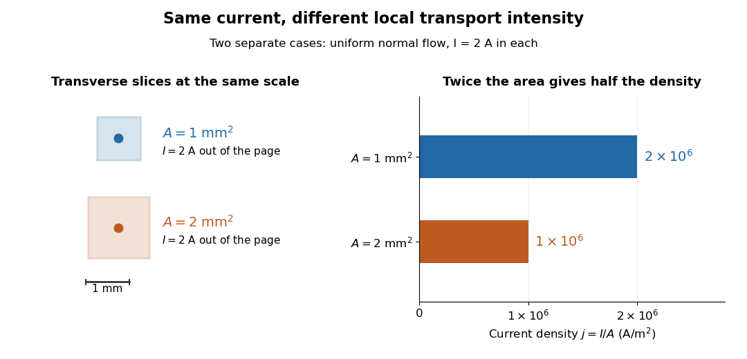
Equal electric current through different wire cross-sectional areas gives different current densities
. Both cases carry with uniform normal current density. The transverse slices use the same spatial scale; the bars compare . Source. Details.
For a toy Electron transport model, stipulate mobile electron number density and drift velocity , with the positive unit normal . Each Electron has electric charge , where the elementary charge is exact in SI. These are defined model inputs, rather than measured parameters of a particular material. [ref] The current density and its magnitude areFor wire cross-sectional area and constant transport over time , this givesThe two minus signs make conventional current point opposite to the Electron drift velocity. A small drift velocity can carry an appreciable electric current because many charge carriers contribute; it does not specify the propagation speed of an electrical disturbance.
An evanescent wave has an imaginary component of its wavevector and therefore decays exponentially in that direction instead of transporting energy away as a propagating wave.
A wavevector points in the direction of phase propagation; its magnitude is the wavenumber and its scalar product with position gives the spatial phase.
An incident SV-wave generally reflects as both an SV-wave and a P-wave. A rigid boundary determines their amplitudes by requiring both displacement components to vanish, while phase matching preserves frequency and tangential wavenumber.
For ,is irreducible over the integers exactly when is prime. Composite gives a geometric factorization; for prime , translation makes the polynomial Eisenstein at .
There are unlisted articles, also show them or only show them.