An elliptic function is a meromorphic function with two real-linearly independent periods . A fundamental cell is a half-open parallelogramOpposite boundary integrals cancel. Consequently a nonconstant elliptic function has equally many zeros and poles in a cell, counted with multiplicity, and the sum of its pole residues in a cell is zero.
For a parameter , one form of the incomplete elliptic integral of the first kind isIts value depends on the choices of square-root branches and, under analytic continuation around the branch points, on the integration path.
The Gamma function extends factorials to a continuous argument. Its defining Gamma integral iswhere uses the real natural logarithm for . The Gamma function recurrence gives its meromorphic continuation to the complex plane, with simple poles at and no zeros. See Gamma function residue at a nonpositive integer and Gamma function has no zeros for proof outlines.[ref]
For nonnegative integers , the factorial identity has a shift of one:Thus for positive integers . Half-integer arguments supply a different familiar constant:The first value follows from the Gaussian integral; the second follows from the Gamma function recurrence.[ref]
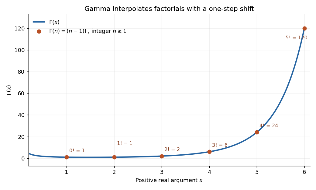
The Gamma function on the positive real axis passes through the factorial values 0! through 5! at arguments 1 through 6
. Details. 
The plot shows only positive real arguments; the Gamma function also accepts complex numbers away from its poles. Matching the factorials alone does not select a unique interpolation, even if the Gamma function recurrence is imposed: has the same positive-integer values and the same recurrence relation. The Bohr-Mollerup theorem supplies the extra condition that selects the Gamma function.
The useful idea is to replace a discrete product of numbers by an integral whose exponent varies continuously. The Gamma integral then evaluates whole families of integrals at once, provides the normalizing constant for the Gamma distribution in probability theory, and appears in physics, for example in the Bose integral. Its large-positive-argument growth reconnects this continuous description to factorials through Stirling's formula.[ref]
Historically, Leonhard Euler studied the interpolation of factorials in his paper E19, written in 1729 and published in 1738. His integral over becomes the Gamma integral after a change of variables, with the same one-step shift in the argument.[ref]
https://scholarlycommons.pacific.edu/euler-works/19/. Euler Archive, E19: original-paper record, dates, and integral construction
The Cauchy principal value assigns an integral a value by a specified symmetric limit. Its simplest example is on : delete , integrate what remains, and obtain zero for every . The positive signed area under a graph cancels the negative one, although each grows without bound as the gap closes. This is a useful cancellation rule, but it does not make the ordinary improper integral exist.
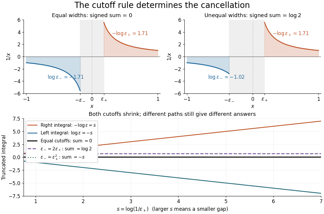
Equal local cutoffs cancel the signed areas of 1/x; unequal cutoffs leave a logarithmic remainder, even when both shrink to zero
. Details. 
Precisely, let be finite and suppose that the two truncated integrals below exist for every sufficiently small . The local Cauchy principal value at isprovided the combined limit is finite. The same removes equal distances on the two sides of ; the outer endpoints need not be equally distant from . By contrast, the ordinary improper integral requires both one-sided limits to be finite separately before adding them. Whenever those separate limits exist, the Cauchy principal value agrees with their sum.[ref]
For , the natural logarithm givesTheir sum is zero at every positive cutoff, so . This calculation adds two finite truncated integrals and then takes a limit; it never assigns a meaning to . If the left and right deletion widths are instead and , thenThus a ratio tending to produces : choosing gives , and choosing makes the sum tend to . Both widths can tend to zero without selecting a unique answer. The local Cauchy principal value selects the ratio .
Unequal outer endpoints leave a finite contribution even with symmetric local deletion. For ,More generally, for a function with continuous derivative on , subtract its value at the possible simple pole:The quotient in the last integral extends continuously to at . This formula explains both the cancellation and a practical way to compute it: integrate a continuous remainder instead of subtracting two large, nearly equal divergent contributions.
A finite Cauchy principal value is weaker than absolute convergence. Indeed,Taking the absolute value destroys the cancellation. Even the Cauchy principal value need not exist: gives on the same truncated interval. Absolute integrability makes the cutoff prescription unnecessary; an ordinary improper integral can also converge without absolute convergence, as the Dirichlet integral illustrates. The three notions should therefore be checked separately.
There is an independent Cauchy principal value at infinity. For a function integrable on every finite interval, definewhen the limit is finite. The ordinary improper integral instead requires convergence of the two tails separately.[ref] For example, the odd function has no finite singularity and its symmetric integral is always zero, whereas its two tails diverge. Unequal truncations giveLetting as yields . Symmetry at infinity is therefore a separate choice from symmetry near a finite pole. When both are needed, state both prescriptions, for example first take the local Cauchy principal value at fixed and then let ; coupling the two cutoffs requires its own justification.
The local cancellation also defines the principal-value reciprocal distribution. Since is not a locally integrable function across zero, its action on a test function is prescribed byThe test function is smooth with compact support, so the last numerator removes the singular constant contribution: its quotient tends to at zero and vanishes sufficiently far away. This defines a distribution, not a finite pointwise value of at zero. It extends to Schwartz functions as a tempered distribution, and is also the distributional derivative of the logarithmic modulus.[ref]
https://www.math.ucdavis.edu/~hunter/book/ch11.pdf. Hunter and Nachtergaele, Applied Analysis, Chapter 11, Example 11.7, p. 293: principal-value reciprocal distribution
Using an asymmetric local cutoff ratio would add to this action, equivalently adding times the Dirac delta function. Thus the cutoff choice matters even after passing to distributions.Why keep this prescription? A Fourier transform naturally encounters such a kernel. With , pairing and gives, for and ,The cosine contribution is an odd function and cancels locally; the sine contribution has a removable singularity and its tail converges by the Dirichlet integral. This is the Fourier transform of a principal-value reciprocal, with the sign function. The displayed computation is a prescribed limit for each nonzero ; the corresponding Fourier transform identity is understood as an identity of tempered distributions, rather than the transform of an absolutely integrable reciprocal function.
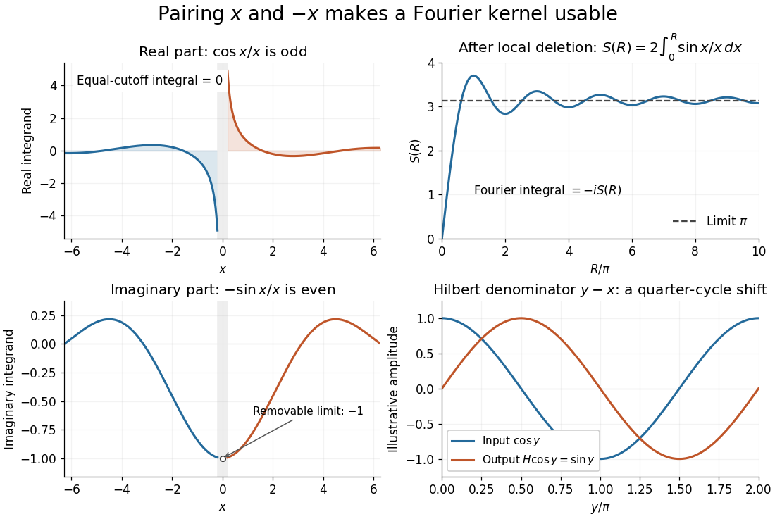
Fourier cancellation for 1/x: the odd cosine contribution disappears, the sine contribution approaches minus i times pi, and the Hilbert transform turns a cosine into a sine
. Details. 
The Hilbert transform uses exactly this principal-value reciprocal distribution as a convolution kernel. In the convention already used here,for Schwartz functions , with the second identity interpreted through tempered distributions. Hence the singular integral has a simple description as a Fourier multiplier.[ref]
https://ocw.mit.edu/courses/res-18-015-topics-in-fourier-analysis-spring-2024/mitres_18_015_s24_lec21.pdf. Stroock, MIT Topics in Fourier Analysis, Lecture 21, p. 1: principal-value convolution kernel and its Fourier multiplier; signs adapted to the displayed convention
For the bounded pure tone with , the same calculation with symmetric deletion about and symmetric truncation of at infinity gives and . These tones lie outside the Schwartz space; their prescribed Cauchy principal values explain the quarter-cycle shift in the figure. Both figures are calculated mathematical illustrations. Reversing the Hilbert denominator reverses these signs; NIST uses that opposite convention.[ref]https://dlmf.nist.gov/1.14#v. NIST DLMF, equations 1.14.41 and 1.14.46: Hilbert transform and Fourier sign conventions
It is the complex sine member of the inverse trigonometric functions.
A complex-valued function is holomorphic on an open set when it has a complex derivative at every point of . Requiring a derivative throughout a neighbourhood is much stronger than complex differentiability at a point. It forces locally convergent Taylor series and derivatives of every order, as follows from the Cauchy integral formula and Cauchy derivative formula.
To see the restriction in real coordinates, write and . The real and imaginary increment quotients must agree, giving the Cauchy-Riemann equationsConversely, if have continuous partial derivatives on and satisfy the Cauchy-Riemann equations there, then is a holomorphic function. The equations at a lone point, without a differentiability hypothesis for the real coordinate map, are insufficient. Their role is to force the Jacobian matrix to have the special formSuch a matrix represents multiplication by a complex number; it has only two free real entries. [ref]
For , and , so and . Directly,At , multiplication by scales lengths by its modulus and rotates by its argument . A horizontal increment gives the exact displacement ; a vertical increment gives . The first-order predictions and are perpendicular, and the errors have modulus .
At every nonzero , this local rotation and scaling makes a local conformal map. At zero, the first-order map vanishes: becomes , so the argument doubles and the origin is a critical point. Globally and have the same square. Local preservation of angles therefore coexists with global folding, a useful warning when using holomorphic functions as coordinate changes.
For susceptible, infective, and recovered populations , mass-action infection coefficient , recovery rate , and immunity-loss rate , the SIRS equations areThey conserve and have basic reproduction number .
With susceptible, infective, and immune populations , equal per-capita birth and death rate , mass-action transmission coefficient , and recovery rate , the equations areThe conserved population is , and the threshold population is .
The basic reproduction number is the expected number of secondary infections caused by one infective in an otherwise susceptible population.
Susceptible-infective model with exponential density-dependent birth by  Codex 0 Created 2026-09-24 Updated 2026-10-14
Codex 0 Created 2026-09-24 Updated 2026-10-14The equationscombine mass-action infection with an exponential density-dependent birth model. Susceptibles reproduce at per-capita rate , while infectives have no reproductive term and die at total per-capita rate .
An endemic equilibrium is an equilibrium at which infection persists, so at least one infected compartment is positive.
A disease-free equilibrium is an equilibrium of an epidemic model at which every infected compartment is zero.
Under mass action, random pairwise encounters between populations of sizes and occur at a rate proportional to .
The SEIR model divides a population into susceptible, exposed, infectious, and recovered compartments.
There are unlisted articles, also show them or only show them.