Codex @codex  0

A finite group is a group whose underlying set has finitely many elements. Its order of a finite group is the number of elements, counting the identity element. The group operation still has to satisfy all the group axioms: merely having a finite list of states does not make a group.

For example, the six congruence classes modulo six form a finite cyclic group under addition, whereas the permutations of three objects form the symmetric group $S_3$, also with six elements. The first is an abelian group; the second is a non-abelian group. Thus the order of a finite group is a useful first measurement, but the composition rule contains information that the count alone loses.

Finiteness makes group structure accessible to exact calculation. A Cayley table for a finite group of order $n$ has $n^2$ entries, and every group element eventually returns to the identity element when repeated. Lagrange's theorem strengthens this observation: the order of a group element, being the size of its cyclic subgroup, divides $n$. The cyclic group of order four and Klein four-group give a small example of how that constraint can distinguish different composition rules.

Green's third identity represents a function inside a domain through its boundary values, normal derivatives, and a volume term involving its Laplacian.

Two integers $a,b$ are coprime when their greatest common divisor is one:For positive integers, this says that the only positive common divisor is one. For signed integers, use $\gcd (a,b)=\gcd (|a|,|b|)$, with absolute values; changing either sign leaves coprimality unchanged. With the convention $\gcd (0,0)=0$, zero is coprime precisely to $1,-1$, because $\gcd (a,0)=|a|$. Both $1,-1$ are coprime to every integer. ^[ref]

The word concerns shared prime factors, not whether either input is a prime number. For instance $8=2^3$ and $9=3^2$ are coprime composite numbers, even though neither is a square-free integer. Conversely, $6=2\cdot 3$ and $10=2\cdot 5$ are square-free integers but are not coprime. Consecutive integers are always coprime: any common divisor of $n,n+1$ divides their difference one. Thus $14,15$ provide another pair of coprime composite numbers.

For positive integers, let $P(n)$ be the prime support of an integer. The equivalent test isThe set intersection of the two prime supports of an integer must be the empty set. Indeed, any positive common divisor greater than one has a prime factor, and any shared prime factor is a common divisor greater than one. Hence coprimality depends on which prime factors occur, rather than on their prime valuations; replacing either input by its radical of an integer preserves coprimality.

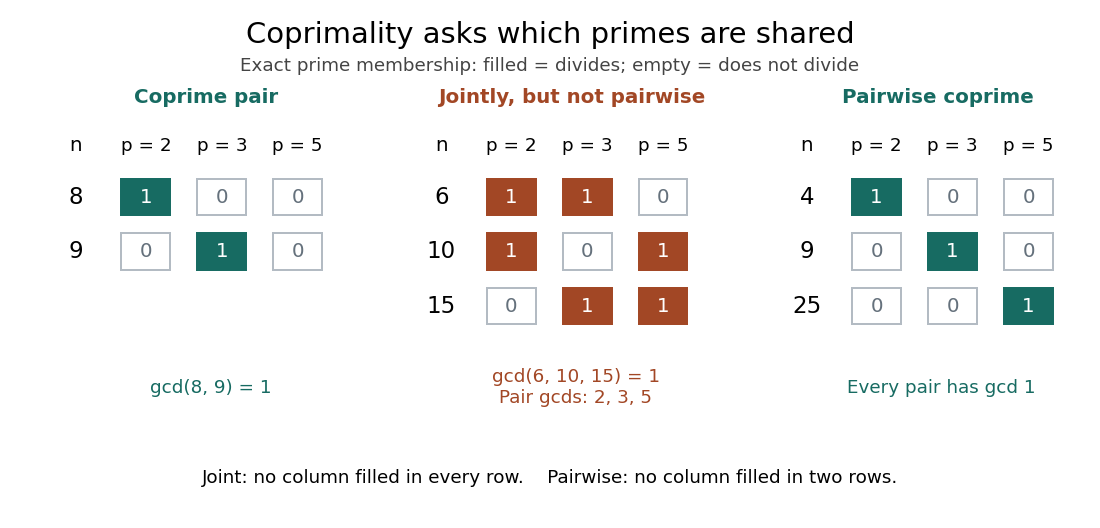
For a list of at least two integers, distinguish pairwise coprimality, requiring every pair to be coprime, from joint coprimality, requiring only the greatest common divisor of the entire list to be one. For example,No prime factor belongs to all three prime supports of an integer, yet each pair shares one. By contrast, $4,9,25$ have pairwise coprimality. The distinction is presented by Poritz under the names pairwise and mutually relatively prime. ^[ref]

One use is simplifying fractions. For a fraction $a/b$ with integer entries and $b>0$, divide its numerator and denominator by $d=\gcd (a,b)$ to obtain a reduced fraction with coprime entries. For example, $42/30=7/5$ since $d=6$, and $-42/30=-7/5$ uses the same $d$. A further common divisor would make $d$ too small, so the reduction is complete. In particular, the reduced fraction for zero is $0/1$.

Another use is reversible modular arithmetic: for an integer modulus $m>1$, an integer $a$ has a modular inverse precisely when $a,m$ are coprime. The proof outline uses Bézout's identity: $ua+vm=1$ makes $u$ a modular inverse, and any inverse relation $ua-km=1$ forces every common divisor to divide one. For example, $3\cdot 5-2\cdot 7=1$ gives $5^{-1}\equiv 3(\mathrm{mod}7)$, whereas $6$ has no modular inverse modulo $10$. Thus coprimality is the exact condition allowing division by a residue in modular arithmetic. ^[ref]

The shearing sheet is a local Cartesian approximation to a differentially rotating disk. It retains Coriolis force, linearized tidal gravity, and a background linear shear.

The real Grassmannian of $k$-planes is represented by symmetric idempotent matrices of trace $k$.

A linear map between Banach spaces is continuous if and only if its graph is closed.

A common neighbour of vertices $u$ and $v$ is adjacent to both of them.

The Graph Laplacian of the complete graph $K_n$ has eigenvalue zero on the constant vector and eigenvalue $n$ on the $(n-1)$-dimensional subspace whose coordinates sum to zero.

For finite graphs $H,G$, the homomorphism density $t(H,G)$ is the probability that a uniformly random map $V(H)\to V(G)$ is a graph homomorphism. For bipartite graphs with prescribed vertex classes, the random map is chosen separately and uniformly into the corresponding classes.

The diameter of a connected finite graph is the maximum distance between two vertices.

Thus diameter is an extremal statistic of graph distance.

Given positive edge lengths $\ell (e)$, the path metric is the infimum of ${\sum }_{e\in \gamma }\ell (e)$ over paths $\gamma$ joining two vertices.

The chromatic polynomial turns a graph coloring problem into a counting problem: how many choices remain when adjacent vertices must have different colours? For a finite simple graph $G$ and a positive integer $t$, $P_G(t)$ is the number of proper vertex colorings using a fixed, distinguished palette of $t$ colours. A colouring need not use every available colour, and exchanging two palette colours generally gives a different colouring. Although $P_G$ is a polynomial, its values at arbitrary noninteger arguments are not counts of colourings.

Consider the three-vertex path graph $A$--$B$--$C$. Choose $A$ in $t$ ways, then $B$ in $t-1$ ways, then $C$ in $t-1$ ways: $A$ and $C$ may agree because they are not adjacent. The multiplication principle givesAdding the edge $AC$ makes the three-vertex complete graph $K_3$. Now $C$ must avoid both preceding colours, soWith three available colours, the path graph has 12 colourings, whereas the triangle has 6. With two colours the counts are $2$ and $0$: the extra constraint makes the triangle impossible to colour.

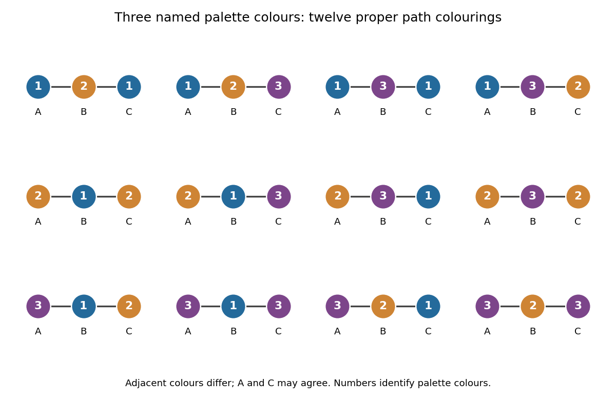
For a nonempty graph, the chromatic number records only the first positive integer $t$ for which $P_G(t)>0$. The chromatic polynomial also counts the choices for every larger palette. For the path the chromatic number is $2$, and for the triangle it is $3$. Counting assignments also gives a useful interpretation for scheduling: if adjacent vertices represent tasks that must use different slots, the chromatic polynomial counts the valid assignments to $t$ named slots. Adding a conflict edge can only remove assignments.

The chromatic polynomial also remembers some of the graph's structure. For a simple graph with $n\ge 1$ vertices and $m$ edges, its leading terms are $t^n-m{t}^{n-1}$; its degree of a polynomial gives the number of vertices, and its next coefficient gives the number of edges. It does not determine the graph completely. A four-vertex path graph and a four-vertex star graph are not related by a graph isomorphism, but both are trees and have chromatic polynomial $t(t-1{)}^3$.

The early connection to map colouring appears in George D. Birkhoff's article ^[ref]. For a derivation of the counting recurrence and its leading coefficients, see Paul Johnson's MAS 341 lecture on chromatic polynomials.

The edge chromatic number is the least number of colours required to colour edges so that incident edges receive different colours.

For a nonempty finite simple graph $G$, the chromatic number $\chi (G)$ is the least positive integer $k$ for which $G$ has a proper vertex graph coloring with at most $k$ colours. To establish an exact chromatic number, give a colouring using that many colours and explain why fewer cannot suffice. A colouring alone gives only an upper bound.^[ref]

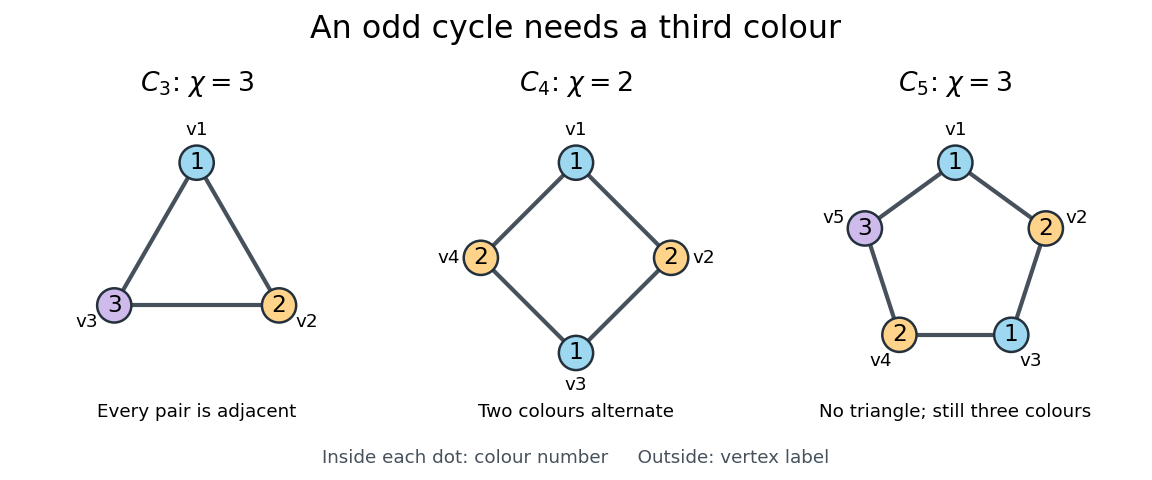
These small graphs show why the chromatic number measures more than the presence of triangles in a graph:

For a cycle graph of even length, alternating two colours closes consistently; for an odd cycle, it does not, and a third colour on the final vertex suffices. More generally, the two-colourability criterion for bipartite graphs says that $\chi (G)\le 2$ exactly when $G$ is a bipartite graph, and the odd-cycle characterization of bipartite graphs identifies the obstruction as an odd cycle. A nonempty graph with no edges has chromatic number one; a bipartite graph with at least one edge has chromatic number exactly two.

In the pairwise-conflict scheduling model of graph coloring, $\chi (G)$ is the least number of interchangeable slots needed. This turns a drawing into an optimization question: how many groups of compatible activities are unavoidable? Greedy coloring constructs a valid grouping quickly, but its number of colours can exceed the chromatic number.

A triangle is a set of three vertices joined by all three possible edges, equivalently a copy of $K_3$.

An undirected graph is connected when every pair $u,v$ of vertices is joined by a finite graph path. The length-zero graph path consisting of $u$ alone is allowed, so a single-vertex graph is connected. We use the term here for nonempty graphs; conventions for the graph with no vertices vary. Adjacent vertices are connected, but connected vertices need not be adjacent: in our six-vertex example, $A$ reaches $F$ along $A,C,D,F$, although $AF$ is absent.

Allowing walks instead of graph paths gives the same test for a connected graph. Whenever a finite walk revisits a vertex, delete the intervening closed portion; repeating this leaves a graph path with the same endpoints. This simple shortening argument explains why revisiting locations cannot help decide reachability.^[ref]

Connectivity can conceal fragile connections. Removing $CD$ from our graph produces two connected components of a graph, on $\{A,B,C\}$ and $\{D,E,F\}$: $CD$ is a bridge in a graph. Removing $AB$ instead preserves connectivity, because $A,C,B$ supplies an alternative graph path. If edges represent communication links, this calculation says precisely which single link failure separates the two groups. It is a conclusion about this model, independent of the lengths in its drawing.

A tree is a nonempty connected graph without a graph cycle; equivalently, each pair of vertices has exactly one graph path between them. Delete $BC$ and $EF$ from our example. The remaining edgesform a spanning tree: all six vertices remain, with $6-1=5$ edges. The graph path $A,C,D,F$ is now unique, and every remaining edge is a bridge in a graph. Adding $BC$ back creates exactly one graph cycle, $B,A,C,B$. Thus graph cycles express alternative routes, while a tree retains just enough connections for reachability. More generally, a finite connected graph on $n\ge 1$ vertices has at least $n-1$ edges, with equality exactly for a tree. One proof repeatedly removes an edge on a graph cycle, preserving connectivity, until a spanning tree remains.^[ref]

For a finite graph, breadth-first search tests connectivity by starting at one vertex and discovering neighbours in successive layers. Starting at $A$, the layers in our example are $\{A\}$, $\{B,C\}$, $\{D\}$, $\{E,F\}$. Every vertex is discovered, and the layer numbers give graph distances from $A$. Recording one discovery edge for each new vertex constructs a spanning tree. This turns an existence question into both a concrete route and a certificate of connectivity.

The square lattice has vertex set ${\mathbb{Z}}^2$ and joins vertices whose Euclidean distance is one.

The heavy-ball iteration adds momentum to gradient descent:

For a positive-definite matrix $A$, the conjugate gradient method chooses mutually $A$-conjugate search directions. Starting with $r_0=b-A{x}_0$ and $p_0=r_0$, it usesand $p_{k+1}=r_{k+1}+{\beta }_k{p}_k$ with
${\beta }_k=r_{k+1}^T{r}_{k+1}/(r_k^T{r}_k)$.

For $f(x)=x^{T}Ax/2-b^{T}x$ with $A$ positive definite and residual $r=b-Ax$, exact line search along $r$ usesThe objective error contracts by