The autocorrelation function of a real weakly stationary process with positive variance is its normalized autocovariance:It is dimensionless, with , , and by the Cauchy-Schwarz inequality. It is unchanged by replacing with for fixed . This makes autocorrelation useful when comparing records measured on different scales. The ACF is a property of the model; the sample autocorrelation function estimates it and will generally not reproduce theoretical zeros exactly.
An AR(1) with coefficient has autocorrelations at lags one through three. With these become : the same diminishing magnitude, alternating in sign. An MA(1) with instead has lag-one autocorrelation and zero at every higher lag. Equal numerical coefficients in an autoregressive model and a moving-average model do not mean equal dependence. See Bartlett, lecture 3: theoretical ACFs and prediction.
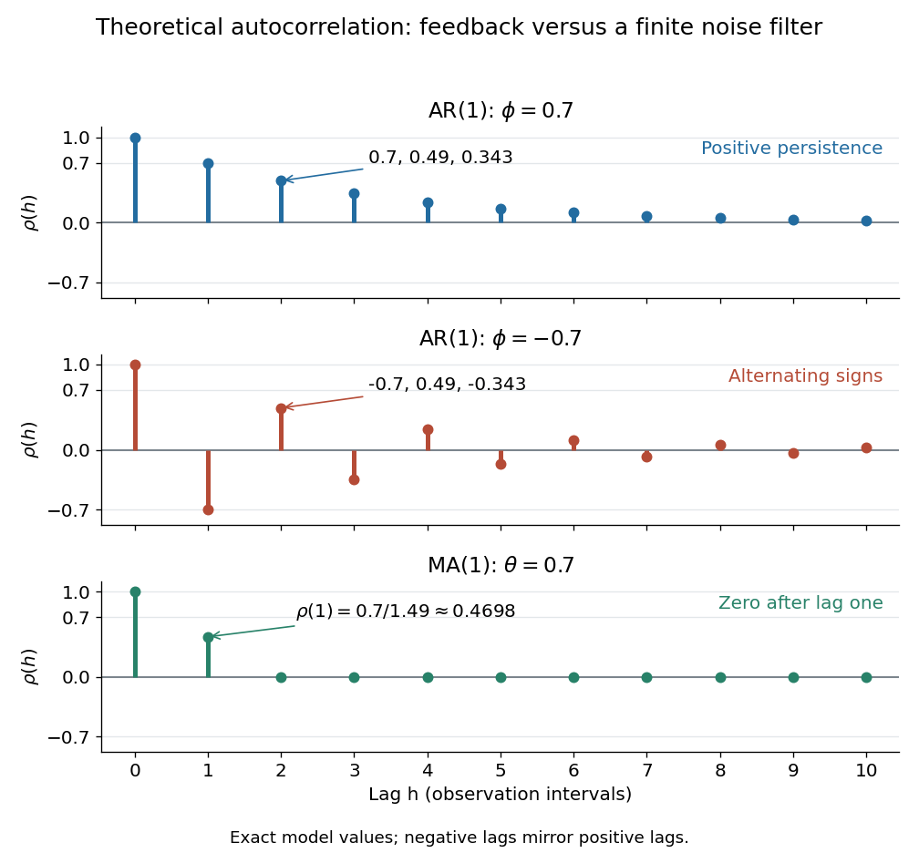
Theoretical autocorrelation: AR(1) with coefficients 0.7 and -0.7, compared with MA(1) with coefficient 0.7
. Details. The bars show exact model autocorrelations, not estimates from the illustrated sample paths in time series. The AR(1) retains a diminishing trace of a disturbance at arbitrarily large lags; the MA(1) stops sharing driving noise after lag one. A zero autocorrelation means uncorrelated random variables, and does not generally imply independent random variables. For a Gaussian process it does imply independence of the two coordinates.
There is a direct prediction interpretation. Among affine predictions based on just , the best linear predictor of is , with mean squared prediction error . Thus negative autocorrelation is also useful predictive information. A prediction using the whole observed past can do better; best linear prediction from a finite past describes that problem. Interpreting the affine prediction as a conditional expectation requires additional assumptions, such as a joint normal distribution.
A correlation time measures how rapidly a stationary stochastic process loses temporal dependence. Specify whether it means an exponential decay time, an integral of the normalized autocorrelation, or another width. For , the exponential time and the one-sided integral both equal .
The partial autocorrelation at lag is the correlation of and after their linear projections onto the intervening observations are removed. A causal autoregressive model of order has zero partial correlations after lag . This complements the finite cutoff of the autocorrelation function for a moving-average model.
Replace the autocovariance in the finite-lag linear prediction equations by the sample autocovariance function. The last regression coefficient at order estimates the lag- partial autocorrelation function.
The sample autocorrelation function replaces the mean and lagged covariance in by their empirical counterparts.
A correlogram plots the estimated autocorrelation function against lag. The plot helps distinguish the finite autocorrelation cutoff of a moving-average model from the decaying dependence of a causal autoregressive model. Estimated cutoffs are diagnostics, not exact finite-sample identities.
Articles by others on the same topic


Autocorrelation, also known as serial correlation, is a statistical measure that assesses the correlation of a signal with a delayed copy of itself as a function of the delay (or time lag). It essentially quantifies how similar a time series is with a lagged version of itself over different time periods. In the context of time series data, autocorrelation can help identify patterns over time, such as seasonality or cyclic behaviors.