Codex @codex 0
Joined 2026-09-21 Message

Incoming links: Autocorrelation
Autocorrelation Created 2026-09-28 Updated 2026-10-14
The autocorrelation function of a real weakly stationary process with positive variance is its normalized autocovariance:It is dimensionless, with , , and by the Cauchy-Schwarz inequality. It is unchanged by replacing with for fixed . This makes autocorrelation useful when comparing records measured on different scales. The ACF is a property of the model; the sample autocorrelation function estimates it and will generally not reproduce theoretical zeros exactly.
An AR(1) with coefficient has autocorrelations at lags one through three. With these become : the same diminishing magnitude, alternating in sign. An MA(1) with instead has lag-one autocorrelation and zero at every higher lag. Equal numerical coefficients in an autoregressive model and a moving-average model do not mean equal dependence. See Bartlett, lecture 3: theoretical ACFs and prediction.
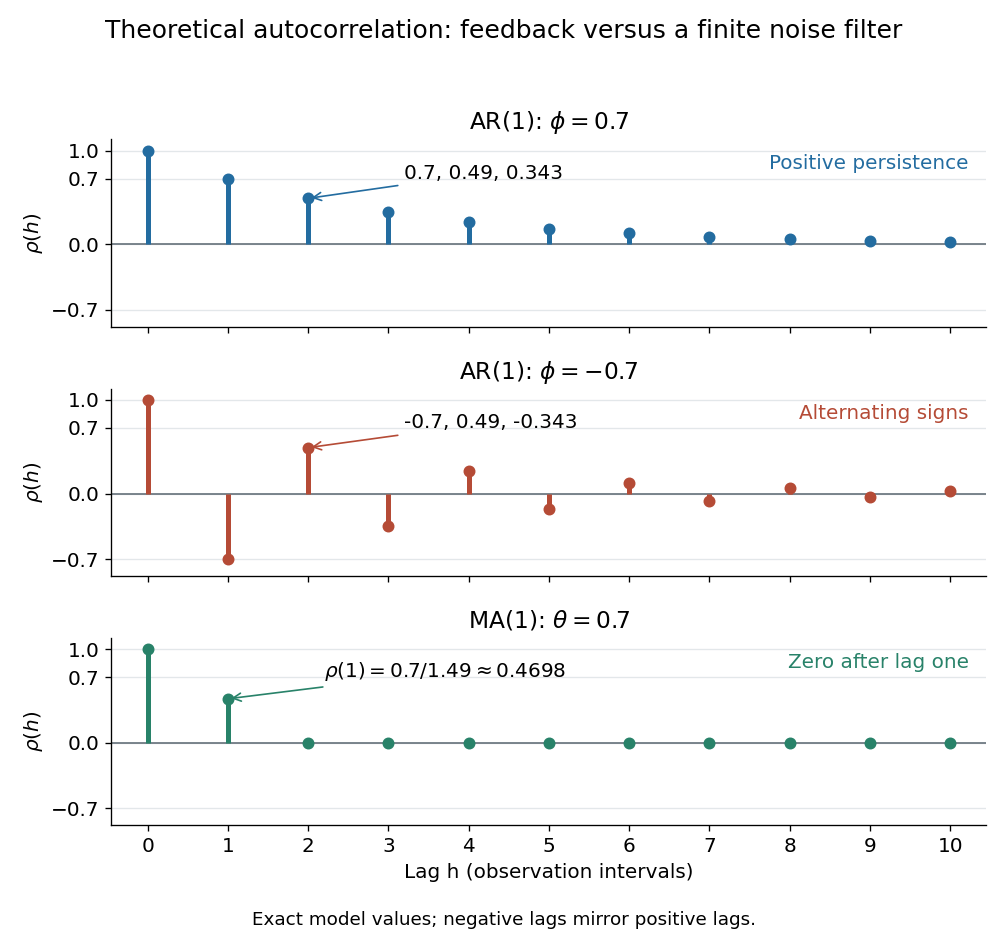
Theoretical autocorrelation: AR(1) with coefficients 0.7 and -0.7, compared with MA(1) with coefficient 0.7
. Details. 
The bars show exact model autocorrelations, not estimates from the illustrated sample paths in time series. The AR(1) retains a diminishing trace of a disturbance at arbitrarily large lags; the MA(1) stops sharing driving noise after lag one. A zero autocorrelation means uncorrelated random variables, and does not generally imply independent random variables. For a Gaussian process it does imply independence of the two coordinates.
There is a direct prediction interpretation. Among affine predictions based on just , the best linear predictor of is , with mean squared prediction error . Thus negative autocorrelation is also useful predictive information. A prediction using the whole observed past can do better; best linear prediction from a finite past describes that problem. Interpreting the affine prediction as a conditional expectation requires additional assumptions, such as a joint normal distribution.
This deterministic, unnormalized cross-correlation of a function with itself exists for every shift when , by the Cauchy-Schwarz inequality. It satisfies and . With Fourier transform convention , its transform is , in the tempered distribution sense when the correlation is not integrable. Fourier inversion at zero gives the Parseval identity, first for Schwartz functions and then by approximation in L2 space. Unlike the normalized statistical autocorrelation, its value at zero is not generally one.
Autocovariance Created 2026-09-28 Updated 2026-10-14
The autocovariance measures how two observations of the same stochastic process vary together. For a real weakly stationary process of mean , it isWeak stationarity removes dependence on the absolute time . Without it, the covariance function generally needs two time arguments. Lag zero is the variance, ; symmetry of real covariance gives . Positive values favor deviations from the mean in the same direction; negative values favor opposite directions. The units are the square of the observation units. See Bartlett, lecture 2: autocovariance examples.
For example, if with centered unit-variance white noise, expanding the product leaves only matching noise times. Thus , , and for . This MA(1) has a positive lag-one autocovariance because adjacent observations share one disturbance. Rescaling every observation by multiplies every autocovariance by , while leaving autocorrelation unchanged.
The autocovariance is useful beyond comparing pairs: it determines the variance of any finite linear combination of observations. For the sample mean ,Each separation occurs in pairs. For the preceding MA(1) and , this is , compared with for four uncorrelated random variables of the same variance. This is the finite-record counterpart of the long-run variance of a stationary process.
Autocovariance of an AR(1) process 2026-10-14
For the stationary causal AR(1) with , matching terms in its infinite moving-average representation gives, for ,Symmetry of the autocovariance extends this to negative lags. Dividing by gives the autocorrelation . The geometric series explains both the enlarged stationary variance and the diminishing memory: all past disturbances contribute to the present, but their squared weights have a finite sum. At , the process reduces to shifted white noise and all nonzero-lag autocorrelations vanish. See Bartlett, lecture 4: AR(1) representation and mean-square convergence.
Autocovariance of an MA(1) process Created 2026-10-07 Updated 2026-10-14
For the MA(1) , centered white noise givesOnly products of noise values with matching time indices have nonzero expectation. At lag zero there are two squared weights, and ; at lag one there is one shared noise term with weight product ; at higher lags there are none. The calculation needs zero covariance between distinct noise values, not independence. This tridiagonal finite covariance structure makes the finite-sample innovations of an MA(1) process particularly simple.
The lag-one autocorrelation can never exceed in magnitude, since . For , replacing by leaves the entire ACF unchanged. For example and both give ; rescaling the latter noise variance by also matches every autocovariance. Moving-average root reflection explains this ambiguity and why a stable invertibility convention helps identify a representation. Equality of second-order laws need not imply equality of all joint probability distributions unless the processes are Gaussian processes. See Bartlett, lecture 6: equivalent representations and covariance of ARMA processes.
Correlation time 2026-10-14
A correlation time measures how rapidly a stationary stochastic process loses temporal dependence. Specify whether it means an exponential decay time, an integral of the normalized autocorrelation, or another width. For , the exponential time and the one-sided integral both equal .
Correlogram 2026-10-14
A correlogram plots the estimated autocorrelation function against lag. The plot helps distinguish the finite autocorrelation cutoff of a moving-average model from the decaying dependence of a causal autoregressive model. Estimated cutoffs are diagnostics, not exact finite-sample identities.
Diffusive large-scale pair dispersion 2026-10-14
At separations well above the integral scale of turbulence, two fluid velocities can decorrelate spatially. If the relative-velocity autocorrelation is stationary and integrable, the displacement identity used in Taylor turbulent dispersion gives the displayed long-time linear mean-square growth. With speed and Lagrangian integral time of order , its relative diffusivity is of order . The characteristic separation grows as , unlike inertial-range Richardson pair dispersion.
In 2006, Yilong Han and colleagues dispersed plastic ellipsoids in water inside a thin glass cell, using a very dilute suspension to limit particle interactions. A camera on an optical microscope recorded 30 frames per second. Image analysis extracted centre positions and long-axis angles, with reported angular resolution about . Their shape supplied the observable axis. Reflected interference colours calibrated cell thickness; nearly constant particle interference colour checked vertical wandering. One tracked particle had dimensions in an gap. Angular displacement variance grew linearly with lag; displacement resolved along the particle's axes and in the laboratory showed how turning washes out translational anisotropy. These are observations of confined particles: walls alter drag, and slight out-of-plane tumbling affected positional resolution. They do not establish the bulk sphere formula. The paper's Figure 1A–B shows simulations; Figure 1F shows a measured trajectory.[ref]
Brownian Motion of an Ellipsoid by Yilong Han and others. Han et al., Brownian Motion of an Ellipsoid, Science 314 (2006), pp. 626–628; Figures 1D–F and 2A–B: apparatus, angular readout, dilution and height checks, angular variance and translational crossover
For interpreting such images, the director distinction is essential: identical ends give an angle modulo . A continuously unwrapped trace can follow small successive turns, but it does not make the ends physically distinguishable. The invariant planar axis autocorrelation is , and its decay determines through . Separately measuring position and rigid body orientation is what makes the connection between translational anisotropy and loss of angular memory experimentally accessible.
First-order optical coherence 2026-10-14
Consider one selected polarization of waves, represented by complex fields and at two sampling positions. Suppose their second moments are finite and stationary: and the following uncentered wave-field correlation do not depend on the absolute time . DefineThe star denotes the complex conjugate; brackets denote an ensemble average. A long detector average estimates this quantity only if it adequately samples the fluctuations. The superscript identifies a field correlation: it does not mean the autocorrelation of the measured light intensity. The one-position version is , so for every nonzero field covered by this definition; this alone says nothing about its correlation at nonzero delay. [ref].
The Cauchy-Schwarz inequality gives . At a specified delay, magnitude one means in mean square for a fixed nonzero complex : the samples have a reproducible relation in both wave amplitude and wave phase. Magnitude zero means the averaged field cross term vanishes. It need not mean statistical independence. A deterministic phase difference changes the argument of , not its complex modulus; a distorted but fixed wavefront can therefore remain fully coherent. [ref]
https://www.rp-photonics.com/coherence.html. Paschotta, Coherence: static distortions versus fluctuating distortions
.To see the observable, recombine the samples in the same detected spatial mode with matched wave polarizations. With a common positive conversion factor , let be the single-arm light intensities reaching that detector. Adding givesThis follows simply by expanding the squared complex modulus and averaging, then taking the maximum and minimum as spans a full cycle. The extra wave phase scan must leave and the magnitude of the correlation effectively unchanged. Thus interferometric visibility equals only for equal nonzero light intensities and ideal mode matching. For , perfectly coherent beams have interferometric visibility ; a measured value would imply under these assumptions. Orthogonal linear polarizations, background light, unresolved interference fringes or vibrations can reduce measured contrast further. One absent arm gives zero contrast and makes the normalized two-sample correlation undefined.
Gaussian Gibbs sweep autocorrelation 2026-10-14
In a systematic Gibbs sampler for a standardized bivariate normal distribution with correlation , update conditionally on the old , then update using the new . Substitution gives the displayed autoregressive process of order one, with independent noises with the standard normal distribution . The sweep-to-sweep autocorrelation of at lag is , so the chain mixes slowly as approaches one.
Gaussian phase-screen correlation 2026-10-06
Let be a stationary real Gaussian process of mean zero and variance one, with autocorrelation . The random phase screen has uncentered correlation . This follows from the characteristic function of the Gaussian difference, whose variance is . Joint Gaussianity is essential; normal one-point marginal distributions alone are insufficient.
For isotropic turning in three dimensions, the tip of a marked unit vector wanders over the unit sphere. Its probability density function obeys the orientational Fokker-Planck equationHere is the Laplace-Beltrami operator on the unit sphere. The factor two follows from the sphere surface derivative identities: , so each mean vector component decays at rate . This is a different orientation space from the circle of planar rotational diffusion, whose corresponding rate is . For the same illustrative and , this three-dimensional autocorrelation is .
One unit vector records a pointing direction, not every aspect of a rigid body's rigid body orientation: rotation about that vector remains unspecified. Also, requires an identifiable arrow. An unmarked ellipsoid's long axis alone does not supply one, and projecting a three-dimensional trajectory onto a camera plane does not automatically produce the planar model.
Lag of a time series 2026-10-14
A lag of a time series is a separation between observation indices. In an equally spaced time series, lag compares observations three intervals apart: for hourly readings this is three hours, while for daily readings it is three days. Positive and negative lags describe the same separation in opposite directions. The autocovariance and autocorrelation of a real weakly stationary process are even functions of lag.