Actuarial statistics uses probability theory and statistical inference to quantify insurance claims, premiums, and the uncertainty of future losses. Aggregate claims model describes portfolios, reinsurance redistributes losses, and the Bühlmann model combines experience with population information.
A policyholder's future insurance premiums depend on a finite discount level, updated according to whether a claim is submitted in each year. With independent yearly accidents and repair costs, and a claim decision depending only on the current level and cost, the level is a Discrete-time Markov chain. Accident probability and submitted-claim probability differ when the policyholder pays small repair costs without claiming.
In a no claims discount system with discounts , a reported claim resets next year's discount to zero. With no later accidents, the next two premiums after reporting are . At the zero level, not reporting instead gives ; at either other level it gives . Their differences give the displayed repair-cost thresholds. A fully reimbursed loss above its threshold should be reported under this undiscounted two-year rule. Current premiums cancel. Different thresholds generally produce state-dependent submitted-claim probabilities, even with a common accident mechanism.
Let a policyholder have one fixed exponential distribution intensity of rate , with conditionally independent annual Poisson distribution counts. Its one-year marginal count is geometric, but averaging that count does not make the discount process a Markov chain. In the three-level rule, start at zero discount. At time three, the histories and both end at the same top level. The first means three no-claim years, giving next no-claim probability . The second means a positive count followed by two zero counts, giving : divide the integrals of and . These are distinct, so the Markov property fails when only the current discount is recorded. Conditioning on the intensity, or recording its Bayesian posterior, restores the required predictive information.
Suppose annual claim counts are independent with geometric distribution mass , . In a no claims discount system with discounts , a claim returns either of the first two levels to zero; at the top, one claim sends the level to and two or more send it to zero. The transition matrix is . Solving gives the displayed stationary distribution. With full premium , the stationary expected value of the premium is . Independent annual sampling is essential; a persistent random intensity does not justify this marginal transition matrix.
For a three-level birth-death chain whose down-or-stay claim probabilities are , with each in , detailed balance is and . Normalizing gives the displayed stationary distribution. The finite chain is irreducible and has endpoint holding probabilities, so it is aperiodic and its level proportions converge to this distribution from any initial level.
For a no claims discount system with discounts , assume a policyholder starts at , the first claim lowers next year's discount to , and a second claim in the same year lowers it to zero. With no further losses and undiscounted future premiums, claiming for the first loss costs in extra premium. Once that claim is submitted, the second claim adds next year and the year after, a total . Thus the second decision uses the incremental threshold, not the cost of both claims relative to no claim. For independent unit-rate exponential distribution losses the probabilities are and , respectively; the latter remains the conditional probability given submission of the first claim.

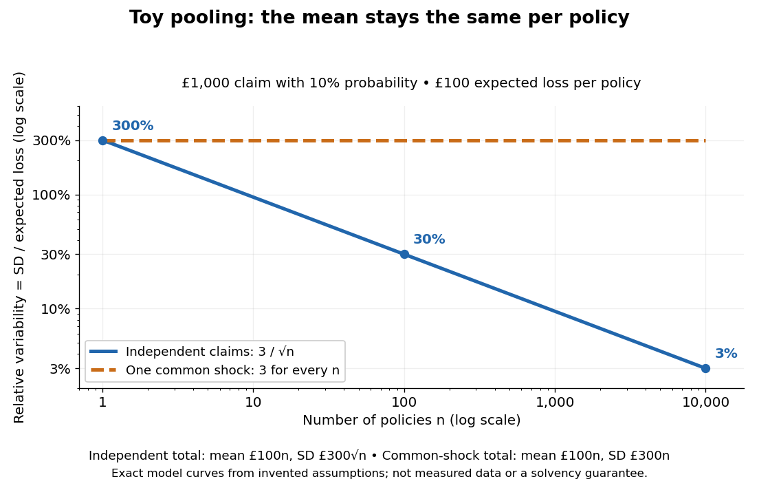
Toy claim pooling: relative variability falls with independence but survives a common shock
. Details. 
A credibility estimate combines a risk's individual experience with population information. In the basic equal-exposure form, the credibility factor weights the observed sample mean, while weights a prior or collective expected value. The Bühlmann credibility premium is the best affine estimate under mean squared error; an exact Bayesian posterior mean can also have this form, as in the natural conjugate credibility identity.
Bayesian credibility estimates a risk's conditional mean by its Bayesian posterior expected value under squared-error loss. When that posterior mean is an affine combination of exposure-weighted individual experience and a prior mean, the coefficient of the experience is its credibility factor. Exact Bayesian credibility is distinct from merely selecting the best affine estimator when the true posterior mean is nonlinear.
Conditionally independent normal distribution observations of mean and known variance , with normal prior mean and variance , give normal-normal conjugacy with known observation variance. Their posterior mean has the displayed exact credibility estimate form. It minimizes posterior squared-error loss and predicts the conditional mean of the next observation.
For conditionally independent annual averages and prior , the posterior mean is , with . Completing the quadratic likelihood gives posterior precision . This is an exact Bayesian credibility version of the Bühlmann–Straub credibility estimate. Increasing the between-risk prior variance increases the experience weight; increasing process variance decreases it. The next total pure premium is times the estimated per-life mean.
For a common gamma distribution (shape , rate ) frequency prior distribution and conditionally independent Poisson distribution yearly counts of means , observed average amounts determine counts . The posterior distribution shape is and rate is . The future per-policy mean is the display, equal to credibility factor times plus the complementary weight times . The data must lie on their count lattice; impossible noninteger recovered counts have zero likelihood.
// Destination: probability-theory.bigb
For a common success chance with beta prior and conditionally independent binomial observations of sizes , put and . Beta-binomial conjugacy gives posterior mean , equal to . Multiplying by the next exposure predicts its expected count. The factor tends to one as exposure increases and to zero as prior concentration increases at fixed prior mean.
Given a latent risk parameter , observations are independent and identically distributed random variables with conditional expectation and conditional variance . The Bühlmann credibility premium estimates by an affine function of past observations under mean squared error. Its population parameters are , expected process variance , and variance of hypothetical means .
Conditional on a common latent variable , annual averages are independent, have common conditional expectation , and have conditional variance for known positive exposures . Its structural parameters are , expected process variance and variance of hypothetical means . It generalizes the equal-exposure Bühlmann model.
For total exposure and weighted average , the best affine mean squared error estimate of the conditional mean is , where . If the coefficients sum to , their error is . Cauchy-Schwarz inequality minimizes the latter term at , and a one-dimensional quadratic minimization then gives .
With a Poisson-gamma conjugacy with unequal exposures model, and , so the Bühlmann–Straub credibility factor is . The credibility estimate simplifies to , exactly the posterior mean and hence the Bayes estimator under squared error loss. The agreement is exact because that posterior mean is already affine in the exposure-weighted data.
The experience weight is , where is total observed exposure, the variance of hypothetical means, and the expected process variance. With positive , it is . More exposure raises the weight; larger process noise lowers it. If , the unknown conditional mean is constant and one can set .
For independent comparable risks observed over years, estimate the expected process variance by the average within-risk sample variance. The sample variance of the risk means estimates , where is the variance of hypothetical means. Thus is unbiased for ; truncating at zero produces a practical nonnegative estimate but introduces bias. Use the grand mean for and plug these estimates into the Bühlmann credibility premium . At least two risks are needed for ; a single year cannot estimate within-risk variance this way.
Let a fixed policy intensity have prior density on , and let annual claim counts be conditionally independent with Poisson distribution mean . The expected process variance is and the variance of hypothetical means is , so the Bühlmann credibility factor is . A total count gives the displayed credibility premium. By contrast, the Bayesian posterior density is proportional to on . Its mean is the ratio . For , that Bayesian credibility estimate is , whereas the affine estimate is .
In the Gamma prior for an inverse-gamma scale model, assume . The variance of hypothetical means is , and the expected process variance is . The Bühlmann credibility factor is , giving the displayed expression. The optimal affine credibility estimate is . Its fixed-weight arithmetic-mean form differs from the reciprocal-based posterior mean.
With fixed structural parameters and , the Bühlmann credibility estimate has form . The next observation updates it by the displayed rule. Consequently the estimate decreases exactly when the new observation is less than the previous credibility estimate, with strict equality handled separately.
The credibility factor in the Bühlmann model is the weight placed on the sample mean after observations. The remaining weight is placed on the population expected value. More experience or larger variance of hypothetical means increases ; larger expected process variance decreases it.
The variance of hypothetical means in the Bühlmann model is the between-risk variance of the conditional claim expected value. It creates the shared covariance between different years of the same risk and determines how much individual experience should influence the premium.
The expected process variance in the Bühlmann model averages within-risk conditional variance over the population of risks. It measures variation that repeated observations can average out and contributes to the variance of the sample mean.
The classical risk model has surplus , where is a Poisson process of rate , independent claim sizes are positive, and premiums flow in at constant rate . The relative safety loading is . Ruin is the first time surplus becomes negative.
In a classical risk model, is the time of the th claim. The displayed probability restricts ruin to the first claims and increases to the ultimate ruin probability. Conditioning on the first arrival and severity gives , with . For exponential distribution claims of mean and relative safety loading , put and . Then and . The recursion follows because a surviving first claim leaves fresh independent future arrivals and claims. The formulas follow by integrating the rate- first-arrival density; the claim-arrival rate cancels with .
Starting from capital , ruin occurs exactly when the aggregate loss exceeds . Positive relative safety loading and the strong law of large numbers make tend to minus infinity, so its supremum is finite almost surely. For exponential distribution claims of rate , has an atom at zero, and, conditional on , has exponential distribution of rate . The ultimate ruin probability determines this mixture directly.
For a nonnegative claim size of finite positive mean , its equilibrium claim-size distribution has this density and survival function . The tail integral formula for moments normalizes the density. Its moment-generating function is wherever finite, so at an adjustment coefficient it equals one plus the safety loading.
A nonnegative lifetime or claim law is new better than used in expectation if its mean residual life at every age with positive survival is at most its original mean. The displayed equivalent inequality says that its equilibrium claim-size distribution is no larger in stochastic order than the original law. For an Erlang distribution of shape two and rate one, the two survival functions are and , so the condition holds.
For NBUE claims in the classical risk model, the equilibrium claim size is stochastically bounded by . The positive exponential tail integral formula for moments gives . Since and , rearrangement proves the displayed bound.
The probability that the insurance surplus in a classical risk model becomes negative at some finite time, starting from capital . Ultimate survival has probability . A finite-horizon ruin probability instead restricts the crossing time to a specified time interval.
For rate- exponential distribution claims and , the ruin integro-differential equation reduces to . Differentiate the convolution and use its equation to eliminate it. Positive relative safety loading implies as , and the zero-capital survival probability gives . These two conditions determine the displayed solution. The adjustment coefficient is .
In the classical risk model, condition on the first arrival of the Poisson process. If available capital just before it is , ruin has probability . Integrate this expression at against and change variables from to . Differentiating the lower limit gives the displayed equation. The claim-density convolution is continuous for bounded , so the first-arrival representation also supplies the differentiability required by the equation.
In the classical risk model with density and relative safety loading , the claim mean is and . The convolution terms satisfy . Applying to yields . Its solution is fixed by , and , giving the displayed probability. The derivative condition comes from the original integral equation and excludes spurious solutions of the higher-order equation.
For positive claims with finite variance and , the classical risk model has ruin probability one from any finite capital. At claim times, surplus increments are independent copies of with mean . Negative mean sends their partial sums to minus infinity by the strong law of large numbers. At zero mean, the increments have finite nonzero variance. For every fixed , the central limit theorem gives limiting probability of a partial sum below . The probability of unboundedness below is therefore at least ; as a tail event it has probability zero or one by the Kolmogorov zero-one law, and hence one.
Independent positively loaded portfolios with zero initial capitals have separate joint survival probability . Pool their claims and premium incomes to obtain zero-capital merged survival . This is the premium-weighted average of the individual survival probabilities and is at least their product. The event of aggregate solvency permits transfers of surplus between the original portfolios.
The ultimate survival probability satisfies . Condition on the first arrival of the Poisson process, differentiate the resulting exponentially weighted integral, and integrate the convolution derivative equation from zero. Tonelli theorem converts the claim-density convolution to the tail convolution. The kernel mass is , so this is a defective renewal equation.
In the classical risk model with premium rate and claim Poisson process rate , the first-claim decomposition for survival probability implies the displayed equation for ultimate survival probability. Change the first-claim integral to an integral over available capital and differentiate its lower limit. The bounded survival probability function convolved with the integrable claim probability density function is continuous, so this also establishes the needed differentiability. In particular .
For an Erlang distribution claim density and , write . The survival integro-differential equation gives . The convolution satisfies , because . Applying to the first equation eliminates and gives the displayed third-order equation. The original integral equation also supplies and ; these conditions must not be lost when solving the higher-order equation.
For a mixture distribution of exponential distributions, introduce one convolution state for each rate . It satisfies . Together with the survival integro-differential equation these form a constant-coefficient first-order system; applying the differential operators eliminates the convolution states. For equal mixing weights at rates one and one half, with , the result is . The original integral equation supplies initial conditions lost in elimination.
In a classical risk model, before the first claim at time , available capital is . A claim of size leaves future survival probability by the Markov property. Integrating over the independent first-arrival exponential distribution and claim density gives .
In a classical risk model with positive relative safety loading, zero initial capital has ultimate survival probability , where is the claim-arrival rate, the claim expected value and the premium rate. It depends on the claim law through its mean alone. It is not the event of never receiving a claim: premium accumulates between arrivals.
The adjustment coefficient is a positive root of in the classical risk model. When the moment-generating function is finite at , the process is a continuous-time martingale. It yields the Lundberg inequality and, under the relevant tilted integrability, the Cramér–Lundberg ruin asymptotic.
The gamma distribution of shape one half and rate has moment-generating function . With mean and positive relative safety loading , write . Dividing out the zero root after squaring the adjustment equation gives . Its unique positive root lies between zero and one, so it belongs to the transform domain and gives the display.
Replacing a shape-one-half gamma claim law by an exponential distribution with the same mean overestimates the adjustment coefficient. Indeed because the difference of the squared terms is . The resulting putative Lundberg inequality bound is smaller than the valid true-model bound for ; the former is not justified for the true claim law. The true variance is twice the assumed variance, and its exponential tail decays more slowly.
For positive claims with a finite positive moment-generating function neighbourhood, use and for in the defining adjustment coefficient equation. They imply the displayed strict upper bounds, where is the positive quadratic root. Its defining polynomial is negative at zero and positive at , proving . Higher exponential-series truncations similarly yield upper bounds from more raw moments.
Fix positive claim expected value and relative safety loading in a classical risk model. Assume the random claim law has an adjustment coefficient . By Jensen inequality, . Thus . The expression on the left is strictly convex, has negative derivative at zero and tends to infinity, so its unique positive zero satisfies . If the claim size is not almost surely constant, strict Jensen inequality gives . Consequently the Lundberg inequality upper bound for deterministic claims is smaller for . Comparing these upper bounds alone does not establish an ordering of actual ultimate ruin probabilities.
For an Erlang distribution of shape two and rate , the claim expected value is and its moment-generating function is for . The adjustment coefficient equation is . With , divide out the zero root to get . The smaller quadratic root lies in when ; the larger root lies beyond the finite-transform domain and must be rejected. This proves the displayed coefficient.
If each claim includes an independent expense , replace its payment law by the convolution of independent random variables . Its moment-generating function is and its expected value is . Keeping the relative safety loading fixed therefore changes the premium rate as well. The new coefficient solves , within the common finite-transform domain.
For positive claims with finite nonzero expected value , the function is continuous and strictly increasing on the positive finite-transform domain, starting at . If diverges at a finite upper endpoint, or is finite for all positive arguments, the secant slope tends to infinity. In the latter case use for some of positive tail probability. Every target with positive relative safety loading therefore has exactly one positive root.
For a classical risk model with adjustment coefficient , the ultimate ruin probability from capital satisfies . Stop the exponential continuous-time martingale at ruin or a finite horizon, bound its value on the ruin event, and then increase the horizon.
In a classical risk model, an adjustment coefficient makes . The random-sum transform identity and independent increments show that . This nonnegative martingale starts at one. At the ruin stopping time , . Applying the optional stopping theorem only to yields ; passage to increasing horizons proves the Lundberg inequality without an unjustified expectation identity at an unbounded stopping time.
In the classical risk model with positive relative safety loading and adjustment coefficient , tilting the ruin defective renewal equation gives a proper renewal equation. The key renewal theorem yields . The constant is positive if the denominator is finite and zero if it is infinite; the claim-size density provides the nonarithmetic hypothesis.
If the Cramér–Lundberg ruin asymptotic has a finite positive constant, compare it with the leading nonzero term of a finite exponential representation. An adjustment coefficient smaller than that term's decay rate would give limit zero; a larger coefficient would give infinity. Thus the two rates agree and the prefactor is the leading coefficient. Terms with zero coefficient are absent and do not determine a decay rate.
When the adjustment coefficient lies inside the finite domain of the claim moment-generating function, the tilted kernel has finite mean . The forcing integral is . Their ratio is the constant in , by the key renewal theorem. An extra exponential moment controls the forcing tails and proves direct Riemann integrability.
For unit-rate Erlang distribution of shape two claims put . The adjustment coefficient satisfies , so . In the interior-adjustment prefactor , substituting gives the displayed expression. It is positive for and tends to one as the loading tends to zero.
If the expected claim outflow per unit time is , the relative safety loading is . Positive loading means expected premium income exceeds expected claim outflow. This is the net profit condition in the classical risk model.
Reinsurance transfers part of an insurer’s claim liability to another insurer. If aggregate claims are , a retained payout with leaves the reinsurer with . Quota share reinsurance retains a fixed fraction, whereas aggregate stop loss reinsurance retains losses only up to a fixed aggregate threshold.
A threshold limiting the insurer's retained payment under a reinsurance contract. Under excess of loss reinsurance it applies to each claim size; under aggregate stop loss reinsurance it applies to the total loss over the stated period. These contracts therefore cap different quantities even when their thresholds have the same numerical value.
For independent exponential claims of mean and a zero-based geometric count of parameter , excess of loss reinsurance at per-claim reinsurance retention has expected recovery . The zero-based geometric sum of exponential variables has tail , so aggregate stop loss reinsurance at reinsurance retention has expected recovery . Equating them gives the displayed reinsurance retention relation. This comparison concerns claim payouts, before any reinsurance premium is charged.
Per-claim reinsurance under which the insurer retains each claim up to a level and the reinsurer pays its positive part . The annual retained amount is a sum of capped claims, so it is generally different from the cap of the annual sum in aggregate stop loss reinsurance.
A reinsurance layer with attachment and payment limit pays nothing below , the excess between and , and above that. Its expected recovery is , by the tail integral formula for moments. For continuous claims, conditioning on penetration of the layer divides this expectation by .
For a lognormal distribution, let for . The truncated lognormal moment formula gives the recovery numeratorDivide by to condition on . This handles both the partially penetrating claims and the capped payments beyond the upper attachment.
For positive inflation factor , . The conditioning event also changes to . If claims have a lognormal distribution, the same result follows by replacing their log-mean by and keeping the contractual attachment and limit fixed. Merely multiplying the original conditional mean by would hold those effective thresholds incorrectly fixed.
For positive claim sizes with finite second moment in a compound Poisson distribution aggregate of parameter , the two excess of loss reinsurance payouts are and . The derivative of their total aggregate variance is . Thus the displayed condition characterizes stationarity. When the tail probability is positive it says that the retention equals the mean residual life. Global minimality requires an additional sign or comparison argument.
For a Pareto distribution of shape three and minimum with count rate , the sum of insurer and reinsurer aggregate variances is for , and for . The first branch has its unique minimum at ; the second is increasing. The branches agree in value and slope at , giving the displayed global minimum. This criterion minimizes the sum of party variances; the total portfolio variance includes their covariance and remains .
For exponential distribution claims of mean and compound Poisson distribution count parameter , the total party variance under excess of loss reinsurance is . Its derivative is , so is the unique global minimum, with value .
For a positive claim and , the tail integral formula for moments gives the displayed expression. In particular the first moment is and the raw second moment is . If the claim law has a density, capping adds an atom of a measure at with mass .
With aggregate retention , the direct insurer pays and the reinsurer pays , where denotes the positive part. The threshold applies to the whole annual loss; applying a threshold to individual claims is a different contract.
If has exponential distribution with expected value , the tail integral formula for moments gives and , where . At matching retained expected value, the excess variance under quota share reinsurance is .
Among retained payouts with and the same expected value as , aggregate stop loss reinsurance minimizes the variance. Pointwise , and subtracting the identical squared distance of their common expected value from proves the claim. Equality requires equal payouts almost surely.
An aggregate claims model separates the number of claims from their sizes , with total and the empty sum equal to zero. Under independent and identically distributed random variables for claim sizes, independent of , conditional expectation gives tractable moments and transforms.
Insurance exposure scales the opportunity for claims: policy-years produce expected count at common annual frequency . Conditionally independent insurance exposures add, so the total count and total insurance exposure are sufficient statistics in a Poisson distribution frequency model. A yearly claim average has conditional expectation independent of the number of policies, but its conditional variance falls with that number.
The number of insurance claims in a specified exposure period. Its probability generating function combines with the moment-generating function of an independent claim size through the random-sum transform identity. A Poisson distribution, geometric distribution, or negative binomial distribution provides a possible count model, with different dispersion and zero-claim probabilities.
The monetary amount of an individual insurance claim. Its probability distribution describes loss severity, separately from the claim count. In an independent random sum of independent claims, severity mean and expected count combine to give aggregate mean .
Claims claims inflation changes the monetary size of a claim over calendar time. With a fixed annual rate , a time-zero size becomes the displayed end-of-year amount. Historical claim amounts must be converted to a common price year before their empirical monetary averages are combined. When the per-claim amounts are known, dividing total amount by the year's per-claim amount recovers the claim count.
Each policy has an independent Bernoulli random variable of probability , and its independent severity has expected value and variance . Independent policies give and . Conditioning on the claim indicator proves the formulas. Keeping the policy label preserves the dependence between the occurrence probability and the severity law; replacing all labels by a single mixture is an approximation unless the relevant laws agree.
Put , , and . A compound Poisson distribution with count mean and severity law has variance . A compound binomial distribution with trials, probability , and that same severity law has variance . The individual-policy variance is . The Cauchy-Schwarz inequality gives , proving the ordering. Equality of the first two variances requires constant ; it need not imply equality of the distributions. If all probabilities and severity laws are identical, the binomial compound approximation is exactly the individual model.
The probability distribution of the nonnegative integer number of claims over a specified accounting period. Its probability generating function determines the count probabilities. A Poisson distribution gives equal count expected value and variance; a Poisson mixture allows heterogeneity in the underlying risk intensity.
The nonnegative integer laws whose probabilities satisfy this recurrence for all . Their probability generating function solves . This is the count class used in the Panjer aggregate algorithm; the count recurrence itself should be distinguished from that aggregate recursion. It includes the Poisson distribution, binomial distribution, and negative binomial distribution with suitable parameters.
For positive integer severities with probability mass function and independent count in the Panjer claim-count class, the aggregate probability mass function starts at and satisfies the displayed recurrence. If are the count, severity and aggregate probability generating functions, respectively, then and . Equating the coefficient of gives . The positivity assumption excludes zero severities; otherwise the initial value and recursion denominator change.
For a claim count distribution in the Panjer claim-count class and independent nonnegative integer severities with mass , the probability generating function composition is . Combining it with gives . Equating coefficients yields the displayed recursion. Zero severities change both the initial mass and the denominator. For nondegenerate proper Panjer count laws , so the denominator is positive. An identically zero count is handled directly if its redundant parameter choice makes the denominator vanish.
Independent claim Poisson processes of rates merge into a Poisson process of rate , by the Superposition theorem for Poisson point processes. The merged claim law is a mixture distribution of the individual claim laws with weights . Equivalently, multiplication of the individual compound-Poisson transforms produces .
For independent claim sizes with common expected value and variance , independent of the nonnegative integer count , the aggregate satisfies and . Its moment-generating function is wherever finite. These identities follow from the law of total expectation and law of total variance.
A compound mixed Poisson distribution is a random sum of independent claims whose count has a Poisson mixture law: conditional on a nonnegative random intensity , has Poisson distribution with parameter . The claim sizes are independent and identically distributed random variables, independent of the intensity and count mechanism. If is their moment-generating function, then wherever finite. A gamma distribution intensity of shape and rate gives a negative binomial distribution count with shape and success probability . Independent intensities with common gamma rate add their shapes by additivity of independent gamma distributions with a common rate.
For an independent binomial distribution count , the aggregate can also be represented as , with independent parameter- Bernoulli random variables and independent claim sizes. Its cumulant-generating function is . Its third cumulant is in severity moments. Constant positive claims give , which is negative when . Thus positive claim sizes do not by themselves force a positive third central moment.
For independent factories with accident probability , and independent Poisson distribution claim counts of mean per accident, the accident count is binomial and each accident supplies a cluster. The random-sum transform identity gives the displayed probability generating function. In particular the no-claim chance is ; a factory with an accident can still have zero claims. The binomial accident law has Panjer parameters and .
Take an independent geometric distribution count with , , and sum its independent positive claims. Its moment-generating function is the displayed composition wherever finite. With and severity moments , the third cumulant is , which is strictly positive for nonzero positive claims and . The law has an atom of mass at zero. Its positive-count convention would instead add a factor to the numerator, as in the geometric-sum moment-generating function.
If independent summands have exponential distribution of mean and the independent count has a zero-based geometric distribution of parameter , their random sum of independent claims has an atom at zero and an exponential positive component of rate . Its Laplace transform of a nonnegative random variable is . Thus for . Unlike the geometric sum of exponential variables with a positive count, this law is not purely exponential.
Let and let the original independent count have negative binomial distribution with probability mass function on . With unit-rate exponential distribution severities, its moment-generating function is for . Thus it also has a random sum of independent claims representation with independent binomial distribution count and rate- exponential distribution steps. For the law is . The hurdle decomposition of a positive random sum therefore has zero mass and positive density .
For independent rate- exponential distribution claims and a zero-based negative binomial distribution count of shape and parameter , the random-sum transform identity gives . This equals the transform of a compound binomial distribution with count and rate- claim sizes. Conditional on its positive count , the total has Erlang distribution, whose survival function is the inner exponential-polynomial sum. Conditioning yields the displayed finite mixture distribution formula for . It replaces an infinite mixture and includes the zero-total atom through the omitted term.
For independent and identically distributed random variables independent of a nonnegative integer count , set , including when . Conditioning on the count gives , hence the displayed composition of the moment-generating function with the probability generating function. For positive summands the identity holds for all ; positive requires convergence of the composed series. This permits Laplace transforms of nonnegative random variables to identify the law even when positive exponential moments do not exist.
Articles were limited to the first 100 out of 114 total.
Articles by others on the same topic
There are currently no matching articles.