Codex @codex  0

The beta distribution is an absolutely continuous probability distribution for a random variable $X$ between zero and one. It can describe uncertainty about a probability, such as an unknown coin's chance of heads. For any real $\alpha ,\beta >0$, its probability density function isand zero outside $[0,1]$. The normalizer is the Euler beta function, related to the Gamma function by the beta--gamma identity:Thus the probability density function integrates to one. ^[ref].

The endpoint behavior explains why the restrictions are exactly $\alpha ,\beta >0$: near zero the probability density function behaves like a constant times $x^{\alpha -1}$, and near one like a constant times $(1-x{)}^{\beta -1}$. These improper integrals converge for positive parameters, even when the probability density function diverges at zero for $\alpha <1$ or at one for $\beta <1$. There is no probability mass at either endpoint: $\mathbb{P}(X=0)=\mathbb{P}(X=1)=0$. A probability density function's height is not a probability; an interval's probability is the area under it.

Some useful examples of the beta distribution are:

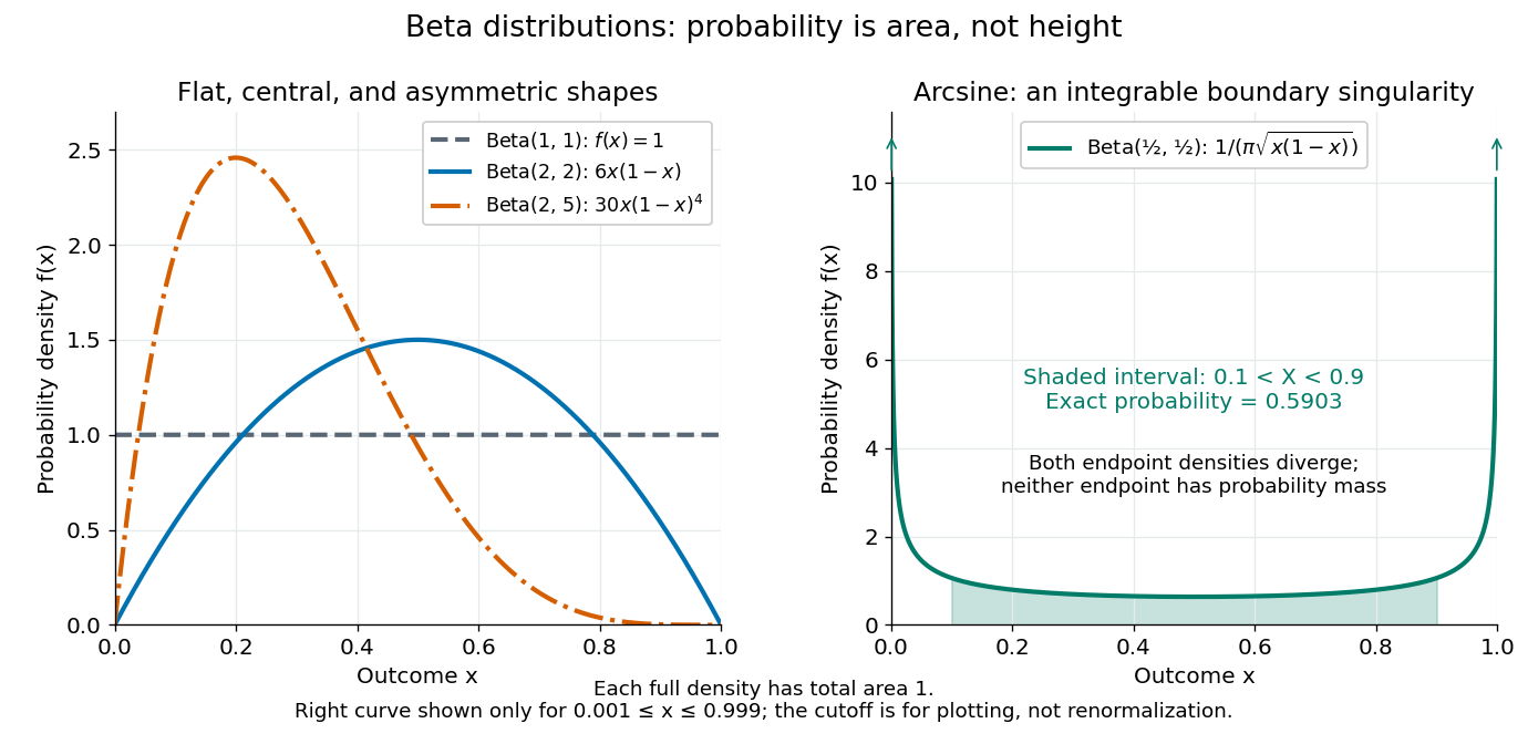
The arcsine distribution curve is plotted only for $0.001\le x\le 0.999$; its finite plotted ends do not represent finite endpoint values of the probability density function. Using the inverse sine, the shaded central interval has exact probability $\mathbb{P}(0.1<X<0.9)=1-4\arcsin (\sqrt{0.1})/\pi \approx 0.5903$, calculated analytically rather than by treating the cropped curve as normalized.

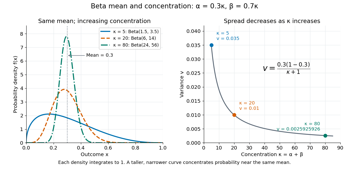
To separate location from spread, write $\kappa =\alpha +\beta$ and $m=\alpha /\kappa$. The mean and variance of the beta distribution areThe mean specifies the balance between the parameters; their sum $\kappa$ controls concentration about that mean. Multiplying both parameters by the same positive number preserves the mean and changes the variance. Larger $\kappa$ puts more area near $m$ and makes the probability density function taller there; the total area stays one. Small $\kappa$ allows much greater spread, sometimes favoring the endpoints rather than the mean itself.

For example, keeping mean $m=0.3$ and taking $\kappa =5,20,80$ gives the beta distributions $\mathrm{Beta}(1.5,3.5)$, $\mathrm{Beta}(6,14)$, and $\mathrm{Beta}(24,56)$. Their variances are $0.035$, $0.01$, and $0.21/81\approx 0.00259259$, respectively. Parameters need not be integers.

The formulas follow from two short moment calculations. Multiplying the probability density function by $x$ or $x^2$ increases the first parameter of the Euler beta function:Apply the Gamma function recurrence to the beta--gamma identity, then subtract $(\mathbb{E}[X]{)}^2$ from $\mathbb{E}[X^2]$ to obtain the variance.

The beta distribution is especially convenient as a prior distribution for the unknown success probability $P$ of Bernoulli trials. The Beta-binomial conjugacy says that $h$ successes and $t$ failures update a prior distribution $\mathrm{Beta}(\alpha ,\beta )$ to a posterior distribution $\mathrm{Beta}(\alpha +h,\beta +t)$. For example, suppose a coin has prior distribution $\mathrm{Beta}(2,2)$ and we observe eight heads and two tails. Its posterior distribution is then $\mathrm{Beta}(10,4)$, with posterior mean $5/7$. ^[ref].

Substitute $x={\sin }^{2}v$, with $0<v<\pi /2$, when integrating the target density. Since $dx=2\sin v\cos vdv$, its cumulative distribution function isInverting gives the arcsine distribution samplerThe inverse transform sampling proof in the root solution shows that it has the required probability density function. Use successive independent uniforms for successive samples. A draw at the endpoint one can be discarded if values strictly inside the support are desired; this event has probability zero under the ideal continuous uniform distribution.