Hall effect

The Hall effect is a transverse electric potential difference produced when an electric current flows through a material in a transverse magnetic field. The contact orientation fixes its measured sign. The Drude conductivity and Hall experiment gives an explicit convention and the limitations of inferring a number density from it.

In an isotropic single-carrier Drude model, let the electric current density point along $x$, with zero transverse current and magnetic field along $z$. The Hall coefficient is $R_H=1/(nq)$ and the longitudinal electrical conductivity is $\sigma =n|q|\mu$, where the charge carrier mobility $\mu$ is positive. Consequently $E_y/E_x=R_H\sigma B=\mathrm{sgn}(q)\mu B$. This signed Hall angle convention describes the angle of the electric field relative to the current; a convention measuring current relative to field has the opposite sign.

A transverse Hall voltage develops when a longitudinal current flows through a sample in a perpendicular magnetic field. With $R_H=E_y/(j_x{B}_z)$, a uniform slab of thickness $t$ along the magnetic field has a signed transverse voltage magnitude set by $R_{H}I{B}_z/t$, with the final sign determined by the chosen voltage leads.

The Hall coefficient relates a transverse electric field to longitudinal current density and transverse magnetic field, with oriented axes as in the displayed formula. Its SI unit is ${\mathrm{m}}^3/C$. For one isotropic Drude model species it is $1/(nq)$; multiple charge carriers need not follow that formula.

In a one-carrier Drude model, the Hall coefficient is $R_H=1/(nq)$. Combining its inferred electron density with atomic density ${\rho }_m{N}_A/M$ gives the displayed number of mobile electrons per atom. The molar mass and mass density must be supplied independently. Multiple bands, anisotropic carrier motion and Hall factors limit this simple interpretation; field reversal helps distinguish the transverse response from voltage offsets.

For one positive carrier population, define $r_H$ by $R_H=r_H/(ep)$ with $e>0$. Different statistical averages of energy-dependent scattering affect hall conductivity and longitudinal electrical conductivity, so $r_H$ need not be one. The measured Hall mobility is ${\mu }_H=\sigma R_H=r_H{\mu }_{\mathrm{drift}}$. Multiple charge carriers require a more general model even before such a correction is made.

In a one-carrier isotropic Drude model, $R_H=1/(nq)$ and an inferred carrier density is $n_H=1/(e|R_H|)$. Dividing by the atomic number density gives an effective Hall count per atom. A noninteger result need not mean a literal fractional count of valence electrons: multiple energy bands, anisotropic Fermi surfaces and different charge carrier mobilities can change the Hall coefficient. In a two-carrier isotropic approximation,Its sign identifies the dominant Hall response rather than necessarily the most numerous charge carrier.

For isotropic electrons and electron holes with positive mobilities, adding their weak-field electrical conductivity tensors and imposing zero transverse total current givesThe Hall coefficient changes sign at $p{\mu }_h^2=n{\mu }_e^2$. Carrier abundance alone does not fix the sign; mobilities enter quadratically. The formula assumes ${\mu }_{e}B\ll 1$, ${\mu }_{h}B\ll 1$, independent semiclassical carriers, and no anomalous Hall contribution.

For fully ionized uncompensated acceptors, $p-n=N_A$ and $np=n_i^2$. If $r_{\mu }={\mu }_e/{\mu }_h>1$, the weak-field two-carrier Hall coefficient is positive when $p>r_{\mu }{n}_i$, giving the displayed sign threshold. A nearly constant Hall coefficient requires a stronger plateau condition. When $N_A\gg n_i$, its relative correction to $1/(e{N}_A)$ is approximately $-(1+r_{\mu }{)}^2(n_i/N_A{)}^2$. Thus specifying only that the coefficient is approximately constant does not define an exact minimum dopant concentration without a tolerance and mobility assumptions.

The quantum Hall effect connects an electrical measurement to a quantum counting rule: a two-dimensional electron gas in a perpendicular magnetic field can exhibit plateaus of transverse electrical resistance. The integer case supplies a resistance scale built from the Planck constant and elementary charge, rather than the sample's dimensions. The fractional quantum Hall effect involves additional many-electron physics.

With unresolved spin and valley splittings, each graphene Landau level has areal degeneracy $4e|B|/h$. Counting carriers from a half-filled zero level yields integer Hall plateaux at filling factors $\pm 2,\pm 6,\pm 10,\dots$. For fixed positive density $n$, plateau-centre fields are $nh/(e\nu )$ and ideal extended-level centres have $B_j=nh/(4ej)$. Localization and level broadening determine finite plateau widths; degeneracy counting does not determine them.

For an integer quantum Hall effect plateau with index $p$ carrying a known current $I$, the true transverse voltage is $I{R}_K/p$. If an offset-corrected instrument displays $D_p$, its gain in volts per displayed unit is $\lambda =I{R}_K/(p{D}_p)$. Independent current and displayed-height errors add in relative quadrature. The Hall-bar width cancels; it enters an electric-field calibration instead. A missing plateau height or an unidentified absolute plateau index prevents a unique numerical gain.

The ratio ${\nu }_{\mathrm{fill}}=n_{s}h/(eB)$ for sheet carrier density $n_s$. Each resolved spin branch has degeneracy $eB/h$ per unit area; an unresolved orbital level can contain two spin branches. A plateau index need not equal total filling everywhere on a finite-width plateau.

On an ideal integer plateau, the magnitude of transverse sheet conductivity is $N{e}^2/h$, where $N$ is a positive integer, while the longitudinal sheet conductivity vanishes. The measured transverse electrical resistance is then $h/(N{e}^2)$. Both statements matter: inverting a conductivity tensor mixes its longitudinal and transverse components, as the quantum Hall conductivity tensor inversion shows.

The von Klitzing constant is $R_K=h/e^2=25812.807459\dots \Omega$. The current SI fixes the Planck constant $h=6.62607015\times 10^{-34}\mathrm{J}\mathrm{s}$ and elementary charge $e=1.602176634\times 10^{-19}\mathrm{C}$ exactly, so $R_K$ is exact; the displayed decimal is truncated. It differs from the historical conventional value $R_{K\text{-}90}=25812.807\Omega$.^[ref]

As an original ideal example, $N=2$ and electric current $I=1\mu \mathrm{A}$ give $|V_H|=I{R}_K/2\simeq 12.9064\mathrm{mV}$. Changing the Hall bar's width changes the transverse electric field required for this electric potential difference, while the ideal ratio $|V_H|/I$ remains $R_K/2$.

Klaus von Klitzing, G. Dorda and M. Pepper reported a silicon MOSFET measurement in 1980. Its gate controlled an semiconductor inversion layer; transverse contacts measured the Hall voltage and separate longitudinal contacts measured dissipation. One sweep held $B=18\mathrm{T}$, $T=1.5\mathrm{K}$ and $I=1\mu \mathrm{A}$ fixed while varying gate voltage. Hall plateaus accompanied small longitudinal voltages. Device-geometry comparisons and high-input-impedance voltage measurements helped test whether contact placement or electrical loading produced the result.^[ref]

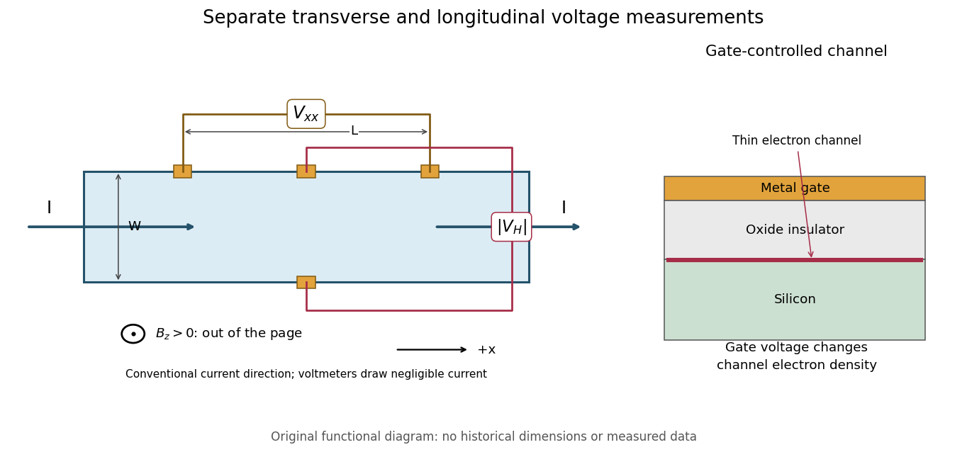
This original functional diagram separates transverse and longitudinal readouts; it does not reproduce the historical device's dimensions. The gate inset explains how a field-effect transistor provides an adjustable two-dimensional electron gas. A longitudinal voltage close to zero is a useful check because accidental longitudinal separation between Hall contacts can otherwise contaminate the transverse measurement.

A Hall bar is a strip with current contacts at its ends and additional voltage contacts along its sides. Opposite-side contacts measure a transverse electric potential difference; same-side contacts at different longitudinal positions measure a longitudinal electric potential difference. Separate voltage leads reduce the influence of current-contact electrical resistance when their input electric currents are negligible.

Voltage contacts separated along the current direction measure longitudinal resistance, even when the device is called a Hall bar. For an approximately uniform rectangular strip, $R_{xx}\simeq {\rho }_{xx}L/W$. Transverse contacts measure $R_{xy}$ instead. Shubnikov-de Haas effect oscillations in $R_{xx}$ need not be Hall-resistance plateaus; in the integer quantum Hall effect, longitudinal minima accompany quantized transverse plateaus.

The degeneracy of a Landau level is $eBA/h$ per resolved internal branch in area $A$. The filling factor $f=n_{s}h/(eB)$ varies continuously. Additional localized eigenstates need not carry bulk transport, allowing an integer plateau over an interval of $f$; a mobility gap need not be an empty spectral gap.^[ref]

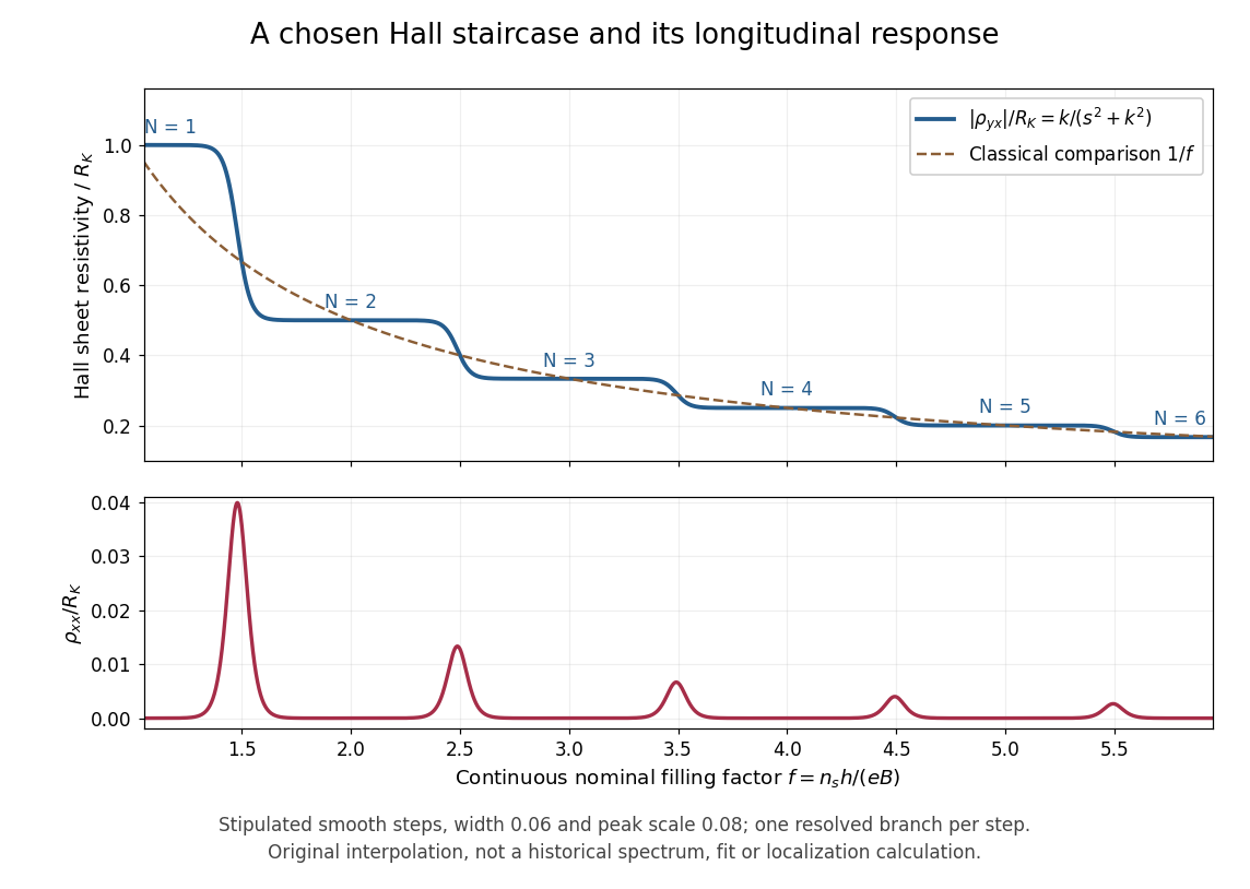
The plot is an original phenomenological construction, not measured data or a calculation of Anderson localization. It stipulates dimensionless transverse sheet conductivity $k(f)=1+\frac{1}{2}{\sum }_{m=1}^5[1+\tanh ((f-m-1/2)/w)]$ and longitudinal sheet conductivity $s(f)=a{\sum }_{m=1}^5{\mathrm{sech}}^2((f-m-1/2)/w)$, with chosen $w=0.06$, $a=0.08$. Both are measured in units $e^2/h$. The quantum Hall conductivity tensor inversion produces $|{\rho }_{yx}|/R_K=k/(s^2+k^2)$ and ${\rho }_{xx}/R_K=s/(s^2+k^2)$. Regions near $k=N$, $s=0$ yield plateaus near $R_K/N$; the model alone does not explain their microscopic robustness. Each step represents one resolved branch, without assuming unresolved spin or valley multiplicities.

Choose conventional surface current density along $+x$, magnetic field along $+z$, and negative electron charge. An isotropic in-plane response has the following sheet conductivity and sheet resistivity tensors for $s\ge 0$, $k>0$:These are matrix inverses, rather than componentwise reciprocals. The sheet conductivity has units siemens, the sheet resistivity ohms. With $K_y=0$, the sign is $E_y/K_x<0$, agreeing with the negative Hall coefficient of a single electron species. Contact polarity can reverse the measured voltage sign, so quote the Hall magnitude. For a homogeneous strip of width $W$ and longitudinal probe separation $L$, $I=W{K}_x$ givesAt $s=0$, $k=N$, these reduce to $R_K/N$ and zero. A nonzero transverse sheet resistivity creates no local Joule heating: the antisymmetric contribution cancels in $\mathbf{E}\cdot \mathbf{K}=(e^2/h)s|\mathbf{E}{|}^2$.

For an original nonideal example, choose $k=2$, $s=0.01$ and $L/W=2$. Then $V_{xx}/I\simeq 129.061\Omega$, while the Hall magnitude is below $R_K/2$ by the relative amount $s^2/(k^2+s^2)\simeq 25.0$ parts per million. An unwanted admixture $0.02V_{xx}$ in the Hall readout would instead introduce approximately $2.58\Omega$. The chosen calculation shows why a small intrinsic tensor correction does not by itself guarantee an accurate contact measurement.

For filled, separated, noninteracting magnetic Bloch bands, the Berry curvature integral over the magnetic Brillouin zone is an integer Chern number $C$, giving $|{\sigma }_{xy}|=|C|e^2/h$. Patches of Berry connection meet through phases with integer windings; continuous gap-preserving changes cannot change $C$. D. J. Thouless, M. Kohmoto, M. P. Nightingale and M. den Nijs developed this band argument; it does not establish the interacting fractional case.^[ref]

A quantum Hall edge state is confined across a boundary but can extend along it and carry electric current. B. I. Halperin related these current-carrying boundary states to quantized Hall transport in a disordered two-dimensional system.^[ref]

A skipping orbit is the semiclassical path of a charged particle whose cyclotron arcs are repeatedly interrupted by a reflecting boundary. The centre of successive arcs advances along the edge. For electrons in a perpendicular positive $B_z$, the opposite sides of a strip carry opposite directed motion. A smooth boundary replaces hard reflections by guiding-centre drift; the quantum counterpart is a quantum Hall edge state.

For locally linear electron confinement potential energy $U(y)$, two Zeeman splitting branches cross the same Fermi energy at positions differing by the energy splitting divided by $|U^{\prime }|$. The expression neglects self-consistent electrostatic screening and exchange interaction enhancement. If the quoted slope is an electrostatic voltage gradient instead of an electron-energy gradient, its magnitude must be multiplied by the elementary charge. A screened compressible quantum Hall edge strip is not a single sharp crossing with an imposed bare slope.

Self-consistent electrostatics allows a partially filled edge Landau level to screen strongly and flatten its effective energy. Such compressible regions alternate with incompressible strips whose chemical potential lies in a gap and across which the potential changes. An externally prescribed unscreened smooth edge misses this redistribution. Temperature, disorder and interactions beyond the electrostatic approximation can change the strip profile.

A depleted potential hill inside a two-dimensional electron gas. In a strong perpendicular magnetic field, closed quantum Hall edge states circulate around it. Coupling these states to propagating edge channels can produce resonant backscattering; Coulomb blockade can substantially alter the single-particle resonance pattern.

A quantum dot is an electron-confining potential well, whereas an antidot is a depleted potential hill. At the same magnetic field, their closed guiding-centre drift has opposite circulation. A series dot needs transmission through two barriers; a side-coupled antidot can connect already propagating quantum Hall edge states and induce backscattering. Both can have discrete energies and charging effects, but a electrical conductance peak or dip depends on lead connectivity rather than solely on the existence of a closed orbit.

A closed antidot edge orbit can tunnel-couple extended channels on opposite edges. When its electrochemical energy aligns with the reservoirs, resonant backscattering reduces conductance from an otherwise transmitting integer plateau. Different connectivity can instead add a transmission path and produce peaks. Gate voltage changes both the orbit and tunnel couplings; charging and spin alter the simplest fixed-area Aharonov-Bohm resonance sequence.

A spin-resolved resonant path adds at most $e^2/h$ to the electrical conductance of directly transmitted spectator channels. Conversely, resonant transfer into a returning edge removes at most $e^2/h$ from an otherwise open channel. For an isolated level, $T(E)={\Gamma }_L{\Gamma }_R/[(E-{ϵ}_d{)}^2+({\Gamma }_L+{\Gamma }_R{)}^2/4]$ reaches one only for equal couplings. Integer offsets follow the channel connectivity and do not follow from a local filling factor alone. temperature, asymmetry, coherent background paths and inelastic processes can change the apparent resonance height and shape.

In an integer-filling charging model, $f$ occupied spin-resolved branches can drive approximately $f$ charge rearrangements per added $h/e$ flux. Two coupled spin branches can therefore yield near-$h/(2e)$ oscillations. This does not change the elementary single-electron flux quantum and is not guaranteed by counting two independent noninteracting spin spectra alone.

For a fixed effective enclosed area $S$, changing the magnetic flux by $h/e$ changes the single-electron Aharonov-Bohm phase by $2\pi$. Gate-dependent orbit area, spin branches and charging can modify the observed conductance-resonance pattern; the lithographic depleted area need not equal the exact enclosed edge-orbit area.

The fractional quantum Hall effect is quantized transverse sheet conductivity at fractional filling factors, produced by interacting electrons. The Laughlin wavefunction describes the sequence $\nu =1/m$, with odd $m$, including $\nu =1/3$.^[ref]

For an original ideal readout example, take a Hall bar on the $\nu =1/3$ plateau with negligible longitudinal sheet conductivity. The quantum Hall conductivity tensor inversion givesHere $R_K$ is the von Klitzing constant; $R_H$ denotes transverse electrical resistance, rather than the bulk Hall coefficient. Thus a fractional sheet conductivity corresponds to a larger transverse electrical resistance. The fraction labels a collective quantum state: it does not mean that each electron has acquired one third of its usual electric charge.

An emergent description of correlated electrons in which an even number of statistical flux quanta is attached to each electron. The resulting effective field can turn selected fractional electronic fillings into integer effective fillings. Flux attachment encodes correlations; it is not attachment of literal external magnetic solenoids to individual electrons.

A fully spin-polarized sea of composite fermions has a Fermi wavevector $\sqrt{4\pi n_s}$. Near half filling its semiclassical orbit radius depends on the residual effective field, not the full applied field. Matching an orbit diameter to a patterned length can produce transport resonances outside an incompressible fractional Hall state. Multiple pattern periods and random/unpatterned controls test that geometric interpretation. Density inhomogeneity and a soft potential can shift or broaden the response.^[ref]

Attach two statistical flux quanta ${\Phi }_0=h/e$ per electron at density $n_s$. For $B>0$, $B^{\ast }=B-2n_s{\Phi }_0=B(1-2\nu )$ and the signed effective filling is ${\nu }^{\ast }=n_s{\Phi }_0/B^{\ast }=\nu /(1-2\nu )$. Inversion gives $\nu ={\nu }^{\ast }/(2{\nu }^{\ast }+1)$. Integer ${\nu }^{\ast }=p$ gives $p/(2p+1)$, while ${\nu }^{\ast }=-p$ gives $p/(2p-1)$. Using nonnegative effective filling instead requires explicitly tracking the effective-field sign. At half filling the mean effective field vanishes.

A family of fractional quantum Hall effect fillings obtained by attaching $2p$ flux quanta and filling $q$ effective Landau levels of composite fermions. Positive integers $p,q$ and the relative effective-field direction specify the branch.

Daniel Tsui, Horst Störmer and Arthur Gossard reported the effect in 1982. They grew gallium arsenide–aluminium gallium arsenide layers by molecular beam epitaxy, separating the two-dimensional electron gas from its semiconductor doping. They cut Hall bars and made indium contacts. Low-field measurements established number density and charge carrier mobility. A perpendicular magnetic field sweep measured transverse and longitudinal sheet resistivities at several temperatures. Cooling sharpened the plateau near $3h/e^2$ and the longitudinal minimum at filling factor $1/3$; integer plateaus provided an internal comparison. The longitudinal minimum remained finite at the lowest temperature: zero-temperature vanishing was unresolved. This established anomalous transport, without directly measuring excitation electric charge.^[ref]

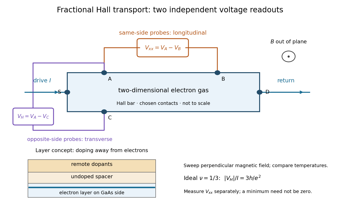
The two readouts test different statements. A single intersection with $R_H=3R_K$ would also occur on the smooth classical relation $R_H=B/(n_{s}e)$ at $n_{s}h/(eB)=1/3$. A quantum Hall plateau instead persists over a magnetic field interval. Comparing transverse and longitudinal signals helps distinguish that plateau from a contact-placement artefact; the quantum Hall conductivity tensor inversion quantifies the contamination when longitudinal sheet resistivity is nonzero.

Later, 1997 shot noise measurements associated with quantum tunnelling at filling factor $1/3$ tested the excitation electric charge separately, finding $e/3$. That is a different observable from a Hall plateau.^[ref]

Robert Laughlin's 1983 variational method uses pairwise zeros to suppress close electron encounters within the lowest Landau level. For aligned spin, odd $m$ gives fermionic exchange symmetry.^[ref]

Here $\mathcal{N}$ enforces wavefunction normalization, ${\ell }_B$ is the magnetic length, and complex coordinates $z_j=x_j-i{y}_j$ describe electrons in a magnetic field $B\hat{\mathbf{z}}$, $B>0$, with the symmetric gauge. Reversing the orientation conjugates the polynomial without changing probability densities. The Gaussian function confines the wavefunction.

The exchange check is especially simple for two electrons. Writing $w=z_1-z_2$, exchange sends $w\mapsto -w$, so $w^m\mapsto (-1{)}^m{w}^m$. An aligned two-electron spin state is symmetric, requiring the spatial wavefunction to change sign. Hence $m=1,3,5,\dots$ works, whereas $m=2$ would give the wrong sign. At a close encounter, the probability density vanishes as $|w{|}^{2m}$: $m=3$ imposes a sixth-order zero, stronger than the quadratic zero at $m=1$. This is the local geometric mechanism for avoiding a large repulsive Coulomb potential energy.

A useful large-$N$ counting outline follows directly from the polynomial. Each complex coordinate has maximum degree $m(N-1)$. A lowest Landau level orbital proportional to $z^k{e}^{-|z{|}^2/(4{\ell }_B^2)}$ has its areal probability density maximum at $r^2=2k{\ell }_B^2$, by differentiating its logarithm. This suggests droplet area $A\simeq 2\pi mN{\ell }_B^2$, neglecting the boundary correction. Dividing $N/A$ by the degeneracy of a Landau level per area, $1/(2\pi {\ell }_B^2)$, gives filling factor $\nu \simeq 1/m$. This counting is a motivation for the fraction, not an independent proof that the wavefunction minimizes the interacting Hamiltonian.

Consider the original two-electron example obtained by taking $N=2$ in the Laughlin wavefunction, with no additional polynomial for the centre of mass. Introduce $Z=(z_1+z_2)/2$, relative complex coordinate $w=z_1-z_2$, separation $r=|w|$, and dimensionless separation $u=r/{\ell }_B$. Since $|z_1{|}^2+|z_2{|}^2=2|Z{|}^2+|w{|}^2/2$, the probability density factorizes:Integrating out $Z$ leaves an isotropic relative probability density. Define $D_m(u)$ per unit dimensionless area and $p_m(u)$ per unit dimensionless separation:The physical areal probability density is $D_m(r/{\ell }_B)/{\ell }_B^2$. The probability of a separation between $r$ and $r+dr$ is $p_m(r/{\ell }_B)dr/{\ell }_B$. The extra $u$ comes from the Jacobian determinant in polar coordinates: a thin annulus has area $2\pi rdr$. Omitting that factor changes the question being answered.

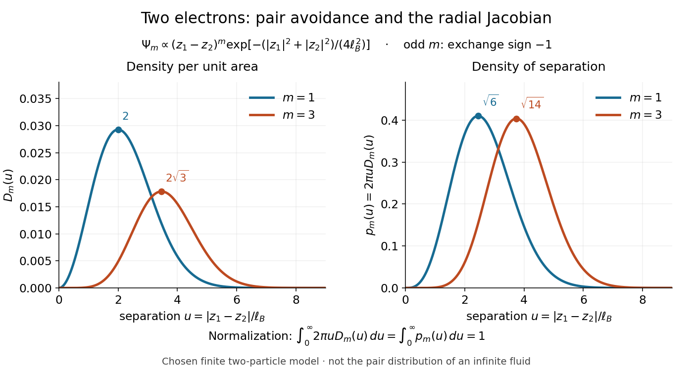
Both wavefunction normalization and the peak shift can be checked exactly. The substitution $t=u^2/4$ gives the Gamma function integralFor $m>0$, logarithmic differentiation givesConsequently the areal maximum lies at $u=2\sqrt{m}$, while the most probable separation lies farther out, at $u=\sqrt{4m+2}$. For $m=1$ these are $2$ and $\sqrt{6}\simeq 2.449$; for $m=3$, $\sqrt{12}\simeq 3.464$ and $\sqrt{14}\simeq 3.742$. The same substitution gives $⟨u^2⟩=4(m+1)$, so the root mean square separations are $\sqrt{8}$ and $4$ respectively. The distinction between a probability density maximum and a radial maximum therefore has a directly calculable geometric origin.

This two-electron model explains exchange and pair avoidance. It does not establish a nonzero many-particle spectral gap, an extended quantum Hall plateau, or the topological properties of a fluid in the thermodynamic limit. Those require additional many-electron reasoning and experimental tests.

A quasihole adds one zero at $\eta$ per electron; its local deficit carries positive electric charge $e/m$.^[ref]

Here is a transport counting outline, conditional on an incompressible quantum Hall fluid. Inserting one magnetic flux quantum $\Delta \Phi =h/e$ slowly compared with $\hslash /\Delta$, where $\Delta$ is the excitation energy gap, produces a circulating electric field by Faraday's law. The transverse sheet conductivity sends a radial electric current whose time integral has magnitudeThe opposite electric charge moves to the boundary, so the total electric charge remains conserved. The counted deficit belongs to a collective quasiparticle; no individual electron has been cut into pieces. The argument assumes the gapped fluid and its Hall response, and is not a consequence of the finite two-electron normalization integral.

An incompressible quantum Hall fluid has a bulk spectral gap against charged excitations; disorder can localize excess quasiparticles.^[ref]