Codex @codex  0

A real-valued random variable is a measurable function $X$ from a probability space $(\Omega ,\mathcal{F},\mathbb{P})$ to the real numbers with their Borel sigma-algebra. More general targets give random elements. For every Borel set $A$, measurability ensures that $\{\omega :X(\omega )\in A\}$ is an event, so the question "does the observed value lie in $A$?" has a defined probability.

The function $X$ is fixed; its input outcome is uncertain. This separates what we measure from how the uncertainty is modeled. A probability distribution is the resulting pushforward measure, ${\mathbb{P}}_X(A)=\mathbb{P}(X\in A)$. A cumulative distribution function, probability mass function, or probability density function describes that measure in an appropriate setting. The random variable and its probability distribution are different objects: the former also retains its relationship to other measurements on the same sample space.

For two independent uniform dice, let $U,V$ record their results and define $S=U+V$ and $M=\max (U,V)$. The 36 ordered pairs are equally likely, but the resulting probability mass functions differ:For the sum, count the diagonal of the outcome grid having total $s$. For the maximum, subtract the $(m-1{)}^2$ pairs with both results below $m$ from the $m^2$ pairs with both results at most $m$. These examples show how a deterministic function transforms a simple input probability distribution into a nonuniform output one.

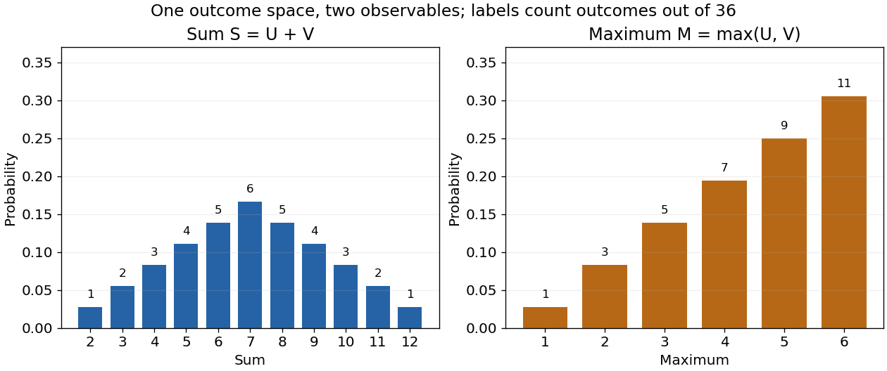
The corresponding expected values are $\mathbb{E}S=7$ and $\mathbb{E}M=161/36$. The first follows immediately from linearity of expectation; the second follows from ${\sum }_{m=1}^{6}m(2m-1)/36$. Neither number must be an attainable result. An expected value describes an average under the probability measure, not a prediction that the next observation will equal it.

The distinction between a random variable and its probability distribution matters for dependence. $U$ and $V$ have the same discrete uniform distribution and are independent random variables. $U$ and a second copy of $U$ also have that same marginal probability distribution, but they always agree. Their joint probability distribution is concentrated on the diagonal; the marginals alone cannot say which relationship holds. This is why a model for several measurements must specify their joint law or an appropriate independence assumption.

Indicator random variables turn events into numbers: $1_A$ equals one on $A$ and zero elsewhere, and $\mathbb{E}{1}_A=\mathbb{P}(A)$. This connects event counting with expected value and variance, and lets tools for random variables answer questions about probabilities. More complicated functions of observations can describe totals, waiting times, or estimation errors using the same framework.

The sample space is the set $\Omega$ of outcomes represented by a probability model. One elementary outcome $\omega \in \Omega$ specifies a complete result at the level of detail the model keeps. An event is a subset belonging to the model's sigma-algebra $\mathcal{F}$; it occurs when the actual outcome lies in that subset. Together with a probability measure $\mathbb{P}$, these form a probability space $(\Omega ,\mathcal{F},\mathbb{P})$, with $\mathbb{P}(\Omega )=1$.^[ref]

Choosing a sample space means deciding which distinctions matter. For two tosses, recording the ordered head-or-tail sequence distinguishes $HT$ from $TH$; recording only the number of heads merges them. Neither representation is automatically wrong, but the second cannot answer a question about which toss was heads. Keeping a detailed sample space and defining a random variable for the desired observation lets several questions share one model.

A sample space alone assigns no probabilities. Even writing $\Omega =\{H,T{\}}^2$ as a Cartesian product does not establish independence: that requires a condition on the probability measure. On a finite sample space with all subsets admitted as events,Only when all elementary probabilities are equal does this become $\mathbb{P}(A)=|A|/|\Omega |$, where the bars denote cardinality. This is the uniform distribution on a finite set, an additional modelling choice.

Sample spaces can also be infinite. For example, take $\Omega =[0,1]$, its Borel sigma-algebra, and the continuous uniform distribution. Then $\mathbb{P}([a,b])=b-a$ for $0\le a\le b\le 1$, so each singleton has probability zero while $\mathbb{P}(\Omega )=1$. Thus an elementary outcome need not carry positive probability, and a continuous model cannot be understood by counting equally likely points. The distinction is developed in zero-probability event and countable additivity.

A sigma-algebra on a set $\Omega$ is a collection $\mathcal{F}$ of subsets such that $\Omega \in \mathcal{F}$, $A\in \mathcal{F}$ implies $\Omega \setminus A\in \mathcal{F}$, and $A_n\in \mathcal{F}$ for all $n$ implies ${\bigcup }_n{A}_n\in \mathcal{F}$. Thus it contains the empty set and is closed under countable intersections as well. This is precisely the closure needed to apply countable additivity without leaving the domain of a measure.

For $\Omega =\{a,b,c\}$,is a sigma-algebra. It describes observations that distinguish $a$ from the pair $\{b,c\}$, but cannot distinguish $b$ from $c$. The power set provides a finer sigma-algebra with all eight subsets. Both are valid; choosing a sigma-algebra records which questions the model can answer.

On the real numbers, the Borel sigma-algebra contains all open sets and everything generated from them by these operations. The Lebesgue measurable sets form a larger sigma-algebra, including all subsets of Borel null sets. Closure under countable unions accommodates constructions involving an entire sequence of observations or approximations.

The sigma-algebra generated by a collection is the smallest sigma-algebra containing all sets in that collection. The displayed intersection is over a nonempty family, since the power set is one candidate. An intersection of sigma-algebras contains the whole space and is closed under complements and countable unions, proving it is a sigma-algebra and establishing minimality.

For example, the half-lines $(-\infty ,x]$ generate the Borel sigma-algebra on the real line. They are Borel, and conversely $(-\infty ,b)={\bigcup }_n(-\infty ,b-1/n]$ and $(a,b)=(-\infty ,b)\setminus (-\infty ,a]$ recover every open interval. Preimages of these half-lines similarly generate the sigma-algebra generated by a random variable.

For a real random variable $X$ on a probability space, $\sigma (X)$ is the smallest sigma-algebra making $X$ a measurable function into the Borel sigma-algebra on $\mathbb{R}$. The collection of all inverse images of Borel sets is already a sigma-algebra, since inverse images preserve complements and countable unions; this proves the displayed formula without completing any measure.

The weak topology and norm topology of a separable Banach space generate the same Borel sigma-algebra. A countable norming family makes every norm ball weakly Borel measurable, and separability makes every norm-open set a countable union of such balls. The reverse inclusion follows because the weak topology is coarser.

There exists a probability measure on $C_0([0,\infty ),\mathbb{R})$ under which the coordinate process is standard Brownian motion, and its distribution there is unique. Construct consistent centered Gaussian finite-dimensional laws with covariance $\min (s,t)$ and use the Kolmogorov extension theorem. The fourth increment moment $3|t-s{|}^2$ supplies a continuous modification by the Kolmogorov continuity theorem. Its independent increments and normal increment distributions are unchanged. Uniqueness follows because coordinate evaluations at rational times generate the Borel sigma-algebra of continuous-path space.