Codex @codex  0

Depth-first search computes minimax search values with much less live storage and naturally supports alpha-beta pruning. A parent's value needs only its current best child value and the next child to visit. Once a child subtree has been evaluated, its internal search nodes can be discarded; a final value cannot usually be computed from a nonterminal frontier alone.

With branching factor

b

and horizon

d

, breadth-first search stores a frontier of order

b^{d}

. A depth-first search implementation storing sibling lists uses

O (b d)

space complexity; lazy successor generation can reduce this to

O (d)

frames plus game-state storage. Both unpruned traversals have

O (b^{d})

time complexity for

b > 1

. Depth-first search also supplies a completed sibling outcome early, allowing alpha-beta pruning to reject later subtrees before generating them.

Past exam of the computer science course of the University of Oxford / 2022 / Artificial intelligence / 3 / c / Solution 2026-10-25

For a finite constraint satisfaction problem with

v

variables, all complete assignments have depth

v

when each step assigns one new variable. Thus the shallowest-solution property of breadth-first search offers no advantage: every complete solution is already at that depth.

Depth-first search with backtracking stores a path and pending choices, using

O (v d)

auxiliary space with ordinary explicit choice bookkeeping, or

O (v)

when each level stores only a current value index. Breadth-first search may store an exponentially large frontier, up to

O (d^{v})

partial assignments. Depth-first search can also combine naturally with immediate constraint propagation and undoing changes. The finite depth avoids the infinite-branch obstruction of unrestricted depth-first tree search. Neither traversal removes the possible exponential time complexity.

Past exam of the mathematics course of the University of Cambridge / 2004 / iii / Paper 33 / 2 / Solution Created 2026-10-03 Updated 2026-10-14

Given a feasible network flow

f

, an original directed edge

(u, v)

has forward residual capacity

c_{uv} - f_{uv}

and a reverse residual arc of capacity

f_{uv}

. A source–sink graph path in this residual network permits an augmentation by the minimum residual capacity along it: increase forward flows and decrease the corresponding reversed flows. Capacities and flow conservation are preserved, and the flow value increases by that amount.

If no residual source–sink graph path exists, let

S

be the vertices reachable from the source. The sink is outside

S

. Every original arc from

S

to its complement is saturated, and every original arc back into

S

has zero flow, since a positive reverse residual arc would make its tail reachable. Conservation therefore gives

∣ f ∣ = \sum_{u \in S, v \in / S} f_{uv} - \sum_{u \in / S, v \in S} f_{uv} = \sum_{u \in S, v \in / S} c_{uv} .

The flow equals this cut capacity, so the max-flow min-cut theorem proves it is maximum.

Termination needs a capacity or path-selection assumption. For integer capacities, starting from zero, every residual capacity and augmentation is integral; each augmentation increases the value by at least one, and the value is bounded by the total source-outgoing capacity. The algorithm therefore terminates. Rational capacities can be scaled to integers. With arbitrary real capacities, unrestricted graph path choices do not guarantee finite termination. A valid uniformly terminating implementation is the Edmonds–Karp algorithm, choosing a shortest residual graph path each time.

Here is why that choice works independently of numerical capacity sizes. Residual distances from the source cannot decrease after augmenting along a shortest graph path. Every newly created residual arc is the reverse of a graph path arc; if it could cause the first distance decrease, its previous distance relation would contradict that decrease. When an arc

(u, v)

is saturated on a shortest graph path,

d (v) = d (u) + 1

. Before the same direction can be saturated again, it must have been restored by a reverse augmentation on a shortest graph path, at which time

d^{'} (u) = d^{'} (v) + 1 \geq d (v) + 1 = d (u) + 2

. Each arc is consequently critical only

O (∣ N ∣)

times. There are

O (∣ A ∣)

arcs and each augmentation saturates at least one, giving

O (∣ N ∣∣ A ∣)

augmentations, each found by breadth-first search in

O (∣ A ∣)

time. Thus the shortest-path Ford–Fulkerson implementation terminates and finds a maximum flow in

O (∣ N ∣∣ A ∣^{2})

arithmetic operations.

For sports elimination by maximum flow, first give the target team all its remaining wins. This cannot hurt its chance to finish strictly ahead: changing a result to favour it also removes a rival's win. Let

w^{*}

be its resulting win count. If any rival already has at least

w^{*}

wins, strict victory is impossible. Otherwise give each unordered pair of rivals

i < j < n

one game node. Its incoming capacity is

g_{ij}

, and its two outgoing arcs go to the participating team nodes. Their capacities may be replaced by the finite number

G = \sum_{i < j < n} g_{ij},

(2)

since no arc can need more than the total number of remaining rival games. Team

i

has sink capacity

w^{*} - w_{i} - 1

An integral flow of value

G

saturates all game-node incoming arcs. Its two outgoing amounts allocate exactly

g_{ij}

wins to the two teams; the team-sink caps keep each rival strictly below

w^{*}

. Conversely any successful completion of the league specifies such a flow. Integral capacities and augmentation give an integral maximum flow, so

the target can win strictly ⟺ the maximum flow has value G,

(3)

after the initial negative-capacity rejection. Each actual game is counted once: making independent nodes for both ordered pairs would double-count it.

The network has

O (n^{2})

nodes and arcs. If each input integer has at most

k

bits, its derived capacities have

O (k + lo g n)

bits. The shortest-path algorithm above uses

O (n^{6})

arithmetic operations, each on integers of polynomial bit length. Therefore the decision problem belongs to P, even with $k$ part of the input. If

k

is fixed, even the basic integral-augmentation bound

O (G ∣ A ∣) = O (n^{4} 2^{k})

is polynomial in

n

. If

k

varies, that particular bound is only pseudopolynomial; it is the shortest-path implementation that establishes polynomial bit complexity.

Past exam of the mathematics course of the University of Cambridge / 2015 / iii / Paper 38 / 4 / b / Solution Created 2026-10-03 Updated 2026-10-14

Run breadth-first search separately in every component of the undirected graph. Give a starting vertex colour zero and each newly discovered neighbour the opposite colour. Reject if an edge joins two vertices with the same assigned colour; otherwise accept after all components have been explored.

If the algorithm accepts, its assignments constitute a graph colouring with two colours. If it rejects, the two search-tree paths and the conflicting edge contain an odd cycle, on which alternating two colours cannot close consistently. Equivalently, a valid graph colouring with two colours fixes the parity of every path from a component's root, so the detected conflict is impossible in a two-colourable graph. The breadth-first search work is

O (∣ V ∣ + ∣ E ∣)

with adjacency lists. Therefore

two-colourability is in P .

This is also the two-colourability criterion for bipartite graphs.

Past exam of the mathematics course of the University of Cambridge / 2016 / iii / Paper 120 / 1 / d / Solution Created 2026-10-03 Updated 2026-10-14

The regular language

L

is nonempty because it represents every element of the group. Find any accepted word

t = a_{1} \dots a_{k}

using breadth-first search in its finite-state automaton. If

t

is the empty word, it already represents the identity.

Otherwise begin with

t \in L

and repeatedly apply the linear-time multiplication in an automatic structure to the letters

a_{k}^{- 1}, a_{k - 1}^{- 1}, \dots, a_{1}^{- 1} .

These letters belong to

A

by symmetry of the alphabet. All intermediate words lie in

L

, and the final word

γ

represents

\overline{t} a_{k}^{- 1} \dots a_{1}^{- 1} = 1.

(2)

Hence an identity representative can be constructed effectively:

γ \in L, \overline{γ} = 1.

(3)

This is a finite preliminary computation depending only on the fixed automatic structure for a group; it uses no test for whether an arbitrary word represents the identity.

Past exam of the mathematics course of the University of Cambridge / 2021 / ii / Paper 2 / 17G / b / Solution Created 2026-09-24 Updated 2026-10-14

If a cubic graph has no cycle of length at most

2 r + 1

, the breadth-first search ball of radius

r

about a vertex is a tree and contains

1 + 3 (1 + 2 + \dots + 2^{r - 1}) = 3 \cdot 2^{r} - 2

vertices. Taking

r = ⌊ lo g_{2} n ⌋

gives a contradiction for a suitable nearby radius, and in particular yields a cycle of length at most

100 lo g n

Choose such a cycle

C

of length

m \leq 100 lo g n

. Removing its vertices deletes at most

3 m

edges. The remaining graph has at least

3 n /2 - 3 m

edges on

n - m

vertices. For all sufficiently large

n

, this exceeds

n - m - 1

, so part (a) says the remainder contains a cycle. It is vertex-disjoint from

C

Past exam of the mathematics course of the University of Cambridge / 2026 / iii / Paper 122 / 1 / a / Solution Created 2026-09-24 Updated 2026-10-14

Explore the connected component of a graph containing a fixed vertex

v

by breadth-first search. If the exploration discovers at least

m

vertices, then before its

m

th discovery at least

m - 1

of at most

mn

tested potential edges must be present. The tests are independent Bernoulli trials with parameter

p = (1 - ε) / n

, so

P (∣ C (v) ∣ \geq m) \leq P (Bin (mn, p) \geq m - 1) .

The binomial distribution on the right has mean

(1 - ε) m

. For

m \geq 2/ ε

, the exponential Markov bound gives

P (∣ C (v) ∣ \geq m) \leq e^{- c ε^{2} m}

(2)

for an absolute constant

c > 0

. The union bound over the

n

choices of

v

now gives

P (max_{v} ∣ C (v) ∣ \geq m) \leq n e^{- c ε^{2} m} .

(3)

Taking

m = C_{ε} lo g n

with

C_{ε} > 2/ (c ε^{2})

makes this probability tend to zero. This proves the subcritical component bound for a binomial random graph.

Past exam of the year 1 of the computer science course of the University of Oxford / 2018 / Functional programming, design and analysis of algorithms / 7 / c / ii / Solution 2026-10-31

Replace breadth-first search by Dijkstra's algorithm from

s

, using the positive edge weights to compute

D (v)

. The strongly connected components, the condensation graph and the reverse-topological order propagation are unchanged, because reachability ignores weights. Only the label assigned to a reachable vertex changes.

With a binary heap, the total time is $O ((∣ V ∣ + ∣ E ∣) lo g ∣ V ∣)$ , including the linear component-processing stages. More specialized priority queues give their corresponding shortest-path bounds. The proof still compares the precomputed distances from

s

; it must not add the weight of a path from

u

to the candidate, which would optimize a different quantity.

Past exam of the year 1 of the computer science course of the University of Oxford / 2018 / Functional programming, design and analysis of algorithms / 7 / c / i / Solution 2026-10-31

First run breadth-first search from

s

to compute each distance

D (v)

. All are finite by hypothesis. Next compute the strongly connected components and their condensation graph

H

. For every component

C

, initialize a representative

b (C)

minimizing

D (v)

over

v \in C

. Process components in reverse topological order, using

b (C) = arg min_{x \in {b (C)} \cup {b (B) : C \to B in H}} D (x) .

Break equal-distance ties consistently, for example by fixed vertex index. Return

b (C)

for every

u \in C

Every vertex of one strongly connected component reaches every other; every reachable different component is reached through some first outgoing edge of

H

. Since

H

is a Directed acyclic graph, reverse topological order has already solved every successor. Induction over that order proves that the representative minimizes

D

over all reachable vertices. This is minimum reachable label propagation.

All stages take $O (∣ V ∣ + ∣ E ∣)$ time and

O (∣ V ∣ + ∣ E ∣)

space with explicit adjacency lists. Retaining parallel component edges is harmless: they can be scanned once each without sorting or deduplication. Reachability here includes the length-zero path, so

u \in P (u)

; this standard convention also makes the requested answer meaningful at a sink.

Past exam of the year 1 of the computer science course of the University of Oxford / 2019 / Imperative programming / 4 / d / Solution 2026-10-25

Use breadth-first search with the supplied FIFO queue, taking one edge to mean one permitted prefix reversal:

def solve(puzzle: Flip): Flip = {
  val pending = scala.collection.mutable.Queue[Flip]()
  pending.enqueue(puzzle)
  while (!pending.isEmpty) {
    val current = pending.dequeue()
    if (current.isIdentity) return current
    var k = 2L
    while (k <= current.game.length.toLong) {
      pending.enqueue(current.flip(k.toInt))
      k += 1L
    }
  }
  throw new IllegalStateException("No solution")
}

val puzzle = new Flip(n)
println("Solving:")
println(puzzle)
val answer = solve(puzzle)
println("Solved:")
println(answer)

The FIFO queue holds pending paths in nondecreasing history length. Initially it holds only the zero-move path. Removing a path at depth

d

and appending its children at depth

d + 1

preserves that order. The inner loop invariant says that precisely moves

2, \dots, k - 1

of the removed state have been appended; its loop variant is

n - k + 1

while the guard holds. The first identity state removed therefore has the minimum possible number of moves. A stack-based depth-first search does not generally have that property.

Termination does not rely on avoiding repeats in this first version. Every permutation can be sorted by prefix reversal sorting: place the largest misplaced value at the front if necessary, flip it into its final position, and repeat on the shorter prefix. This constructs a route of at most

2 (n - 1)

moves. Each search depth has finitely many paths, with at most

n - 1

children per path, so breadth-first search reaches some solution depth after finitely many expansions. This gives a finite bound on remaining expansions before the first solution even though the repeated-state path tree is infinite. The one-element game is already solved. Repeated paths can nevertheless make time and storage enormous; part (e) removes that waste.

Past exam of the year 1 of the computer science course of the University of Oxford / 2019 / Imperative programming / 4 / e / Solution 2026-10-25

Give each solving session a shared visited set keyed by immutable snapshots of permutation contents, for example game.toList, and insert the initial snapshot immediately. Have all successor objects refer to that same session's set. The refined flip first constructs the candidate state; if its key is present, return None. Otherwise add the key immediately and return Some(candidate). The search enqueues only Some results. Keys must compare contents rather than array identities, and a fresh solving session must start with a fresh visited set.

Marking at generation time prevents the same state from being queued repeatedly, including the immediate cycle made by applying the same reversal twice. First discovery in breadth-first search already has minimum depth, so discarding later discoveries cannot remove a shorter solution. The graph now has at most

n!

admitted states. If only cycles along one path were to be rejected, a path-local set would suffice, but it would still repeat states reached by different paths; the shared session-wide set avoids both kinds of repetition. Public game fields must not be externally mutated while their states are being searched.

Past exam of the year 1 of the computer science course of the University of Oxford / 2022 / Imperative programming (resit) / 7 / b / ii / Solution 2026-10-25

Use the heap-numbered binary tree with root label zero and children

2 k + 1, 2 k + 2

. Its strict descendants in breadth-first search order are $1, 2, 3, \dots$ . A machine-safe Node[Int] version stops at the largest representable label:

class NumberNode(val label: Int) extends Node[Int] {
  require(label >= 0)
  def children(): Iter[Node[Int]] = new Iter[Node[Int]] {
    private var candidate = 2L * label.toLong + 1L
    private val last = candidate + 1L
    def hasNext: Boolean = candidate <= last && candidate <= Int.MaxValue
    def next(): Node[Int] = {
      require(hasNext)
      val answer = new NumberNode(candidate.toInt)
      candidate += 1L
      answer
    }
  }
}

val traversal = breadthFirst(new NumberNode(0))
var expected = 1
while (expected <= 1000) {
  assert(traversal.hasNext)
  assert(traversal.next().label == expected)
  expected += 1
}

The arithmetic is widened before computing child labels, so no negative wrapped labels occur. Repeated hasNext calls should not skip nodes; a leaf root should produce immediate exhaustion, and uneven finite trees should retain sibling order across parents. A fresh second traversal should start again at one.

Literal unbounded increase is impossible with the bounded Int type. For a genuinely infinite test, change the label and child arithmetic to BigInt; the same construction then has no representational endpoint. The shown finite-prefix test already exercises lazy traversal without allocating the entire very large Int-labelled tree.

Past exam of the year 1 of the computer science course of the University of Oxford / 2023 / Functional programming, design and analysis of algorithms / 5 / c / Solution 2026-10-25

First run breadth-first search, ignoring weights, to obtain the minimum number of edges

h (v)

from the source to each reachable vertex. Then compute weighted distances only along edges that advance one breadth-first layer:

d[source] = 0; all other d[v] = infinity
for u in nondecreasing BFS-layer order:
    for each outgoing edge (u,v):
        if h[v] == h[u]+1:
            if d[u]+w(u,v) < d[v]:
                d[v] = d[u]+w(u,v)
                predecessor[v] = u

Unreachable vertices keep distance

\infty

. For an undirected graph, scan both orientations of each edge.

To justify discarding other routes, a shortest path can be taken simple because every weight is positive. A simple path of

r \leq n - 1

edges has weight in

[r, r (1 + 1/ n)] \subseteq [r, r + 1) .

Every path with at least

r + 1

edges weighs at least

r + 1

. Consequently every minimum-weight path must also have the minimum possible number of edges: this is minimum-hop dominance for nearly unit weights.

A minimum-hop path to

v

uses exactly

h (v)

edges. Every prefix of such a path must itself have minimum hop count, since replacing a longer prefix by a shorter one would shorten the whole route. Hence it advances from layer

j

to layer

j + 1

at every step. The retained edges form a Directed acyclic graph, ordered by

h

. The displayed dynamic programming recurrence therefore finds the cheapest of all minimum-hop paths, which by the preceding bound is a true shortest path.

Figure 1.
Disjoint weight bands for simple paths with different hop counts
. **Details**.

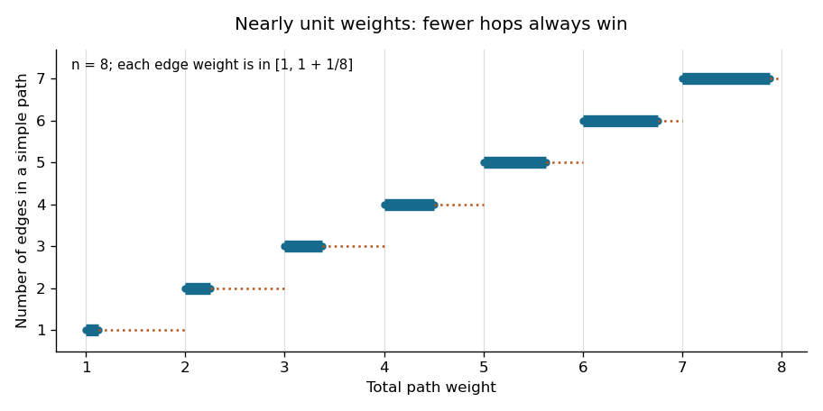
With an adjacency list, both the breadth-first search and the layer-ordered relaxations take $O (n + m)$ time and $O (n + m)$ total storage, where

m = ∣ E ∣

. The queue order from breadth-first search already supplies the layer order; no sorting or priority queue is needed. This improves the usual

O ((n + m) lo g n)

binary-heap Dijkstra bound and is linear in the input size.

Prefix reversal Created 2026-10-24 Updated 2026-10-31

Reverse the first

k

entries of a sequence and leave its suffix unchanged. On a permutation, this is a bijection on positions and is its own inverse: performing the same reversal twice restores the state. The nontrivial moves have

2 \leq k \leq n

. With unit-cost moves, the resulting state graph supports a breadth-first search for a minimum-move solution.

Prefix reversal sorting Created 2026-10-24 Updated 2026-10-31

To sort a permutation using prefix reversals, work backwards through final positions. On an active prefix of length

m

, find its largest value. If it is already at the final position, shorten the active prefix. Otherwise move it to the front with one reversal if necessary, then reverse the entire active prefix to put it last. Already settled suffix positions are untouched.

The settled suffix is a loop invariant, and active-prefix length decreases to one. This proves reachability of the identity permutation in at most

2 (n - 1)

nontrivial flips. The construction is a finite upper bound, not a promise of minimum length; breadth-first search can find the minimum for small instances.

Rooted tree Created 2026-09-28 Updated 2026-10-14

A rooted tree is a tree with a distinguished vertex, its root of a tree

r

. Choosing

r

turns connections into a hierarchy: every other vertex has a unique parent in a rooted tree, the preceding vertex on its graph path from

r

. Conversely, the vertices whose parent in a rooted tree is

v

are the children in a rooted tree of

v

. Choosing the root of a tree changes this description, while the underlying edges remain the same. Arrows towards the root of a tree can encode the relationship, as in MIT's counting notes; the undirected tree itself needs no arrows. ^[ref]

In the seven-vertex tree above, choose

r = 1

. The levels, grouped by graph distance from the root of a tree, are

{1}

{2, 3}

{4, 5, 6}

{7}

. The children in a rooted tree of

2

are

4, 5

, and the parent in a rooted tree of

7

6

. Choosing

r = 7

instead makes the levels

{7}

{6}

{3}

{1}

{2}

{4, 5}

: now

6

has parent in a rooted tree

7

, reversing their relationship. All six edges survive.

This hierarchy supports structural recursion: process the smaller rooted trees below each vertex, then combine their results. A depth-first traversal of a tree explores one branch before returning; breadth-first search processes successive levels. The lowest common ancestor identifies where two routes from the root of a tree last coincide. For

4, 5

it is

2

when

r = 1

. A binary tree imposes an additional restriction on children in a rooted tree; a general rooted tree has no such bound.

Shortest path problem 2026-10-14

The shortest path problem asks for a graph path from a source vertex

s

to a destination vertex

t

minimizing its total edge weight. Here

w_{e}

is the cost of traversing edge

e

, and costs add along the graph path. If no route exists, its shortest-path distance is

\infty

. With nonnegative edge weights, deleting cycles in a graph from a walk never increases its cost, so repetitions cannot improve the optimum.

Consider the undirected graph with vertex set

V = {A, B, C, D}

and the six edge weights

w_{A B} = 4, w_{A C} = 1, w_{CB} = 2, w_{B D} = 1, w_{C D} = 5, w_{A D} = 10.

Each edge can be traversed in either direction at the same cost. The direct graph path

A, D

costs

10

;

A, B, D

costs

4 + 1 = 5

;

A, C, D

costs

1 + 5 = 6

. The cheapest graph path is

A, C, B, D

, costing

1 + 2 + 1 = 4

. The remaining graph path

A, B, C, D

costs

11

, exhausting the possibilities without repeated vertices.

Figure 1.
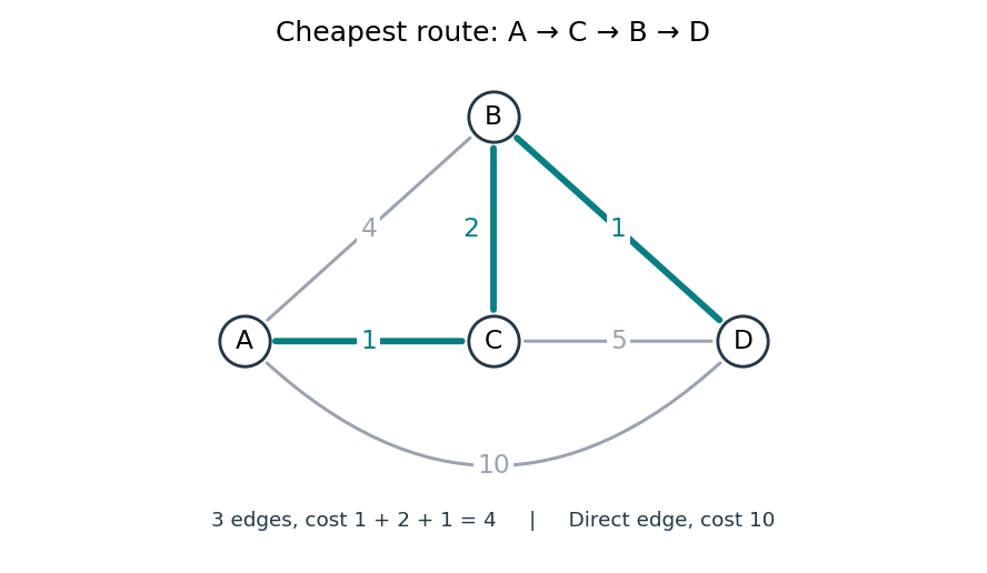
The shortest path problem: three highlighted edges cost less than the direct connection
. **Details**.

Thus fewest edges and least total cost are different objectives. Breadth-first search minimizes the number of edges, which suffices when every edge has the same positive cost. Unequal nonnegative costs call for the Dijkstra algorithm. On a map, weights might be minutes rather than kilometres: a longer-looking route can arrive sooner. This is why a weighted graph separates the network's connections from what a particular journey costs.

Spanning tree Created 2026-09-24 Updated 2026-10-14

A spanning tree of a connected graph

G

is a subgraph that is a tree and contains every vertex of

G

. Its edges must come from

G

. For finite

G

n

vertices, every spanning tree has

n - 1

edges, the minimum possible number preserving reachability between all locations. This makes a spanning tree a compact certificate that the original graph is connected. A minimum spanning tree additionally minimizes a specified total edge weight; merely selecting a spanning tree supplies no such optimization. ^[ref]

Let

G

be our seven-vertex tree with edge

57

added. It has seven edges and a graph cycle. Removing

57

gives the original spanning tree

T

; removing

13

instead gives another spanning tree

T^{'}

. Both retain all seven vertices and six edges, but their graph distances differ:

d_{G} (5, 7) = 1

, whereas

d_{T} (5, 7) = 5

. In

T^{'}

d_{T^{'}} (5, 7) = 1

but

d_{T^{'}} (1, 3) = 5

, along

1, 2, 5, 7, 6, 3

, compared with

d_{G} (1, 3) = 1

. Preserving reachability permits longer journeys; breadth-first search can preserve graph distances from one chosen starting vertex.

Figure 1.
Two spanning trees preserve reachability but change different graph distances
. **Details**.

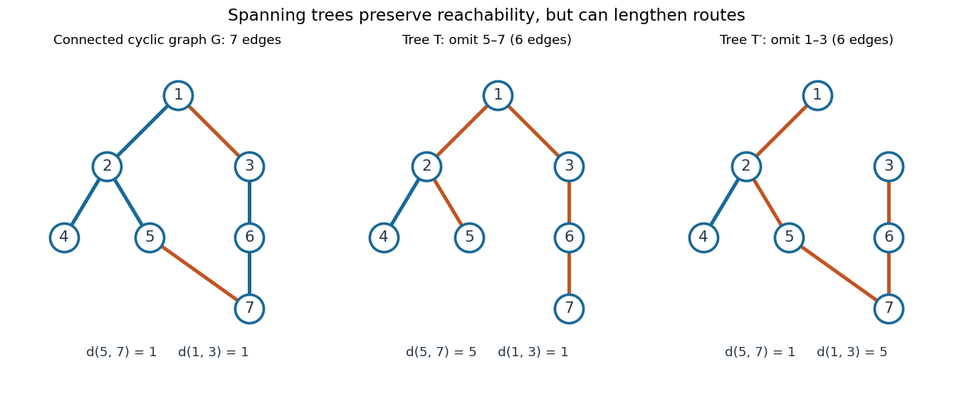
To construct a spanning tree, repeatedly delete any edge on a graph cycle. Its endpoints remain joined through the rest of that graph cycle, so the deletion preserves connectedness. Finiteness ensures that this stops at a connected acyclic graph. Conversely, adding an omitted edge to a spanning tree creates its unique fundamental cycle; deleting any other edge on that graph cycle produces another spanning tree. The displayed exchange replaces

13

57

. ^[ref]

Stack (data structure) 2026-10-13

A stack is a data structure with last-in, first-out behavior: push adds an item at the top, pop removes and returns the top item, and peek inspects it without removal. Push

A, B, C

: successive removals return

C, B, A

. Inspection and removal require a nonempty stack, or a specified empty-case result. A linked list whose head is the top supports all three operations in

O (1)

worst-case time under constant-cost pointer operations and allocation. The stack interface itself does not fix these costs. ^[ref]

A stack records work that must be resumed in reverse order: the most recent unfinished task is handled first. Depth-first search uses this discipline to finish a newly entered branch before resuming the older branch that led to it. Breadth-first search uses a FIFO queue to resume the oldest pending vertex instead. Both are small interfaces whose removal rule changes the shape of a graph search.

Uniform labelled tree generation 2026-10-14

For

n \geq 2

, choose

n - 2

independent random variables, each with the uniform distribution on a finite set

{1, \dots, n}

, and decode their values as a Prüfer sequence. Every sequence has probability

n^{- (n - 2)}

, and the bijection gives each labelled tree the same probability. This produces a uniform spanning tree of the complete graph without repeatedly proposing sets of edges and rejecting those that fail to be trees. It supplies random inputs for testing implementations of breadth-first search and a tractable model of random connections. ^[ref]

This distribution is uniform over fixed-label trees, rather than over unlabelled trees. With four labels, the star graph shape has probability

4/16 = 1/4

and the path graph shape has probability

12/16 = 3/4

. Also, for a fixed label

v

, the Prüfer degree formula gives

de g_{T} (v) - 1 \sim Binomial (n - 2, 1/ n), E [de g_{T} (v)] = 1 + \frac{n - 2}{n} = 2 - \frac{2}{n} .

Here the binomial distribution counts the independent code positions equal to

v

. The expected value agrees with the average vertex degree from the degree-sum formula. Individual labels have the same distribution by symmetry, though their vertex degrees are constrained together by their fixed sum. When

n = 1

, simply return the single isolated vertex.