Codex @codex  0

Control theory studies how to choose control inputs for a dynamical system so that its plant output follows a reference signal, despite control disturbances and imperfect knowledge of the controlled plant. A controller turns the available information into a control signal. The design must consider both the resulting response and stability theory: a rule that corrects a small mismatch can still produce growing deviations if the interconnection is badly chosen. ^[ref]

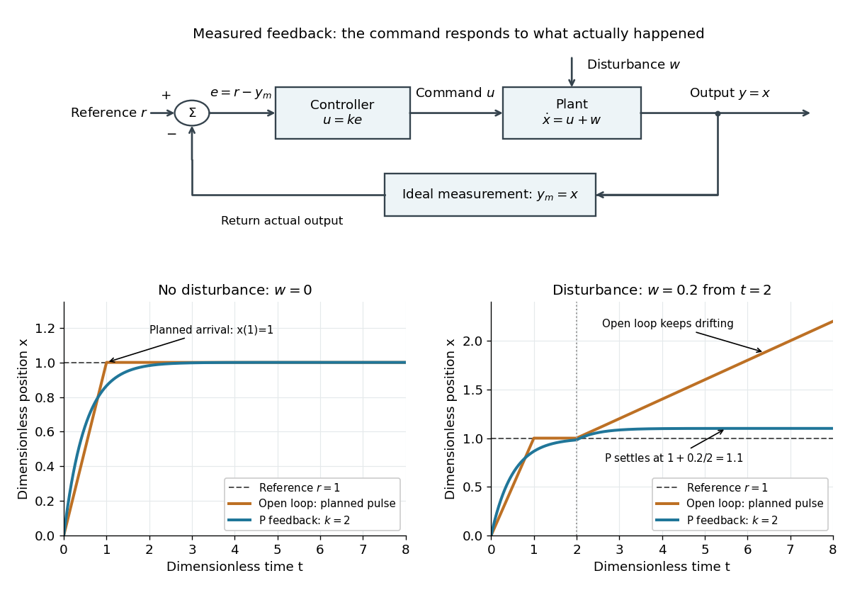
The central distinction is informational. Open-loop control executes planned commands; feedback control uses the measured output of the actual controlled plant to update those commands. A reference signal can describe a destination, while control disturbances describe influences that the controller did not command. A model can predict where the controlled plant should be; measurement tells the controller what actually happened. The authors provide a free full-book PDF through ^[ref].

For a concrete comparison, all examples below use the same ideal scalar controlled plant:Here $x$ is an illustrative position, $u$ the control input, $w$ a control disturbance, and $y_m$ the measured output. Both $x$ and $t$ are dimensionless quantities; the numbers are chosen to expose the mechanism, with no empirical interpretation. The ordinary differential equation says that the present control input and control disturbance accumulate into $x$. The measured output equals the entire state only in this ideal example; a general plant output need not reveal the entire state.

Measurement noise is a fluctuating contribution to measurement error. An additive model for a measured output is $y_m(t)=y(t)+n(t)$, where $y$ is the actual plant output. A controller using feedback control can react to $n$ as though it were a change in the plant output. This effect is absent from the ideal noiseless examples under control theory; an errors-in-variables model represents a related distinction between latent quantities and their noisy observations.

An electrical engineer whose research includes optimization and control theory.^[ref]

Homepage: www.mit.edu/~parrilo/

A physiological integrator combines regulatory inputs to select a response; it need not perform the mathematical integral action used in control theory. In thermoregulation, the hypothalamus participates in combining internal and skin signals. The term describes a role, which can be distributed across interacting biological cells, rather than a mandatory single comparator.

The controlled plant is the part of a control theory model that receives the control input and produces the plant output, including the mechanism that applies the command. The controller is specified separately. In the illustrative ordinary differential equation $\dot{x}=u+w$, the controlled plant accumulates the control input and control disturbance; it does not itself choose $u$.

A transfer function packages the response of a linear time-invariant system into a rule for turning a plant input into a plant output. Instead of solving a differential equation separately for every signal, take a Laplace transform, multiply by $G(s)$, then transform back. This also makes it possible to compare slow and fast oscillations through the continuous-time frequency response.

Here consider a continuous-time, causal, finite-dimensional linear time-invariant system with one plant input $u(t)$ and one plant output $y(t)$. With every initial state set to zero, its transfer function is defined byThe ratio $G(s)=Y(s)/U(s)$ is used where $U(s)\ne 0$ in a common Laplace convergence region; $G$ describes the system, independently of that particular plant input. Zero initial state matters: stored motion or another nonzero initial condition can contribute to the plant output even when the plant input vanishes. ^[ref]

The first-order low-pass filter below shows the same transfer function predicting both a step and a sustained sinusoid. Its pole gives a decay rate, its value at zero gives the eventual gain, and its values along the imaginary axis give the continuous-time frequency response. These descriptions make a useful bridge between a physical relaxation model and control theory calculations.