Codex @codex  0

Source notation assumption: the second printed $V_{p3}=3000\mathrm{m}{\mathrm{s}}^{-1}$ is interpreted as $V_{s3}=3000\mathrm{m}{\mathrm{s}}^{-1}$. Otherwise the S-wave velocity in salt is not supplied, and this part and the salt S-wave calculations below would have no numerical answer. Retain the printed densities, including the unusually low salt value, rather than silently replacing them with typical rock properties.

With that interpretation, Snell law for elastic waves gives

P-wave seismic impedance is $Z_P=\rho V_P$. In layer order limestone, sandstone, salt,The salt's larger P-wave seismic velocity is exactly offset by its smaller printed density, so the second interface has no P-wave seismic impedance contrast in this stipulated model.

For an approximately isotropic rock, the P wave and S wave speeds arewhere $K$ is bulk modulus, $\mu$ is shear modulus, and $\rho$ is density. Five important controls are:

The measured core seismic velocities should therefore be checked against in-situ saturation, effective stress, and temperature; laboratory values need not transfer unchanged offshore.

Take horizontal interfaces, water depth $h_w=50\mathrm{m}$, and sediment thickness $h_s=20\mathrm{m}$. Both source and receiver are just below the sea surface. Every angle below is measured from the vertical interface normal. Snell's law preserves the horizontal seismic ray parameterA basement seismic head wave of speed $V_h$ has horizontal propagation at the basement interface, so $p=1/V_h$. The two possibilities are:

The water supports only P waves. At oblique incidence the seabed can convert a P wave into an SV-wave in the sediment, and the return SV-wave can convert back to a P wave in the water. Further seismic mode conversion can occur at the basement. Thus the down-going and up-going sediment legs can independently be P or S. The S entries refer to SV-waves; a fluid P wave source in this two-dimensional isotropic geometry does not excite the decoupled SH-wave sector.

Let $L_h\ge 0$ be the distance travelled along the basement interface. For sediment legs $a,b\in \{P,S\}$,The first-appearance distance is the limiting value at $L_h=0$:

For example, the unconverted P branch gives $2(50+20)\tan 36.870^{\circ }=105\mathrm{m}$. The earliest geometrically permitted basement P seismic head wave is the doubly converted path with sediment S legs, at approximately $90\mathrm{m}$. The corresponding basement S family first appears at approximately $297\mathrm{m}$. These limiting distances describe existence of ray branches; a finite detectable wave amplitude also depends on conversion efficiency and acquisition noise.

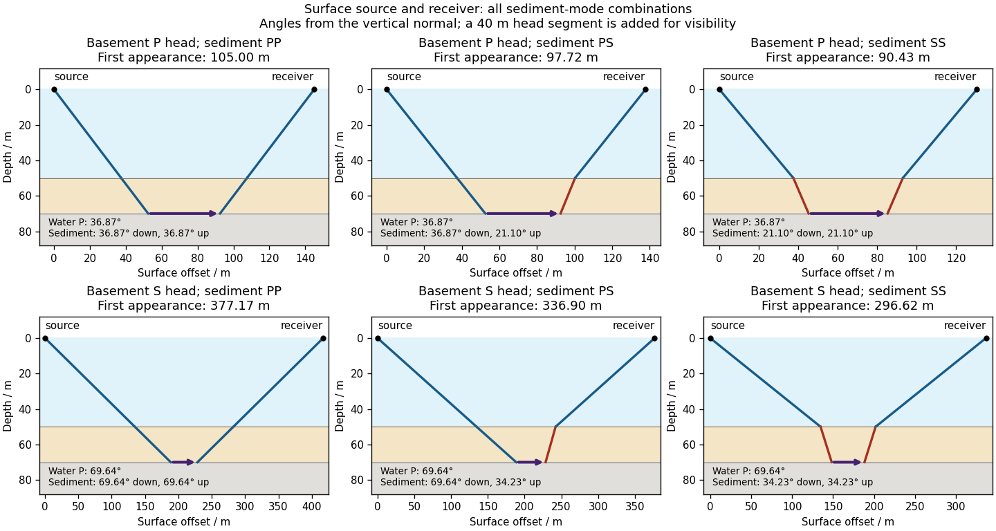
There is no separate finite-distance P head wave at the water–sediment interface: $V_{p,w}=V_{p,s}=1500\mathrm{m}{\mathrm{s}}^{-1}$, so the nominal critical angle is $90^{\circ }$, and a ray from a source 50 m above the interface cannot reach it at finite horizontal distance. Nor can the slower sediment S speed, $900\mathrm{m}{\mathrm{s}}^{-1}$, support a seismic head wave launched from water: it would require $\sin {\theta }_w=1500/900>1$. A seismic reflection still exists at the seabed because the densities, hence the acoustic impedances, differ.

First appearance and first arrival differ. For each permitted branch the travel time isThe all-P basement P branch has $t_h=x/2500+0.0746667\mathrm{s}$. It overtakes the direct water P wave, $t_d=x/1500$, only at $x=280\mathrm{m}$. The converted P-head branches have larger seismic intercept times, so even where they exist at shorter offsets they are later arrivals. The S-head branches are likewise later than the all-P P-head branch wherever they exist in this model. Reflections and layer reverberations can supply additional later phases.

A gravity anomaly is the difference between observed gravitational acceleration and a specified reference prediction after defined reductions. A free-air gravity anomaly, a Bouguer gravity anomaly, and a residual local gravity anomaly differ because they remove different reference contributions. State the reference ellipsoid, datum, reference density, and regional trend before interpreting an anomaly as a subsurface geophysical density contrast.

On land, tie gravimeter observations to a gravity base, calibrate them, correct instrumental drift and Earth tides, and determine station latitude and elevation accurately. Subtract latitude-dependent normal gravity $\gamma (\phi )$. Reduce to the reference elevation using a positive free-air correction for a station above that datum: about $+0.3086h\mathrm{mGal}$ for $h$ in metres. A simple Bouguer gravity anomaly then subtracts attraction of the intervening rock slab and adds the conventional terrain correction:with all acceleration terms expressed consistently. In SI units $1\mathrm{mGal}=10^{-5}\mathrm{m}{\mathrm{s}}^{-2}$.

At sea, also correct vessel-motion effects, especially the Eötvös correction from east–west vessel motion and Earth rotation, and vertical ship acceleration; average or filter the moving-platform data appropriately. GPS navigation and tide information specify position and measurement height. Sea-surface measurements give a marine free-air gravity anomaly after motion, latitude, tide and height reductions. A marine Bouguer gravity anomaly additionally allows for measured bathymetry and the replacement of low-density water by reference rock; the simple water-column replacement correction is positive, $2\pi G({\rho }_{\mathrm{ref}}-{\rho }_w)H$, relative to the sea-surface free-air value. A consistent three-dimensional bathymetric correction is preferable near irregular coasts. Remove a justified broad regional field if the intended quantity is a residual anomaly of the local body.

For a wide horizontal Bouguer slab replacing surrounding basement, use the density contrast $\Delta \rho ={\rho }_{\mathrm{sed}}-{\rho }_{\mathrm{base}}$, not the absolute sediment density:Take downward attraction as positive. The negative anomaly therefore requires $\Delta \rho <0$. With $\Delta g=-40\mathrm{mGal}=-4.0\times 10^{-4}\mathrm{m}{\mathrm{s}}^{-2}$, $h=3000\mathrm{m}$, and $G=6.67430\times 10^{-11}{\mathrm{m}}^3\mathrm{k}{\mathrm{g}}^{-1}{\mathrm{s}}^{-2}$,soThis is the requested Bouguer slab approximation: a flat observation surface, laterally infinite constant-thickness material, uniform average geophysical density contrast, and a regional anomaly already removed. The actual basin in Figure 1 narrows downwards and is finite. For a fixed maximum thickness, finite width reduces the central anomaly magnitude, so this calculation can underestimate the true magnitude of the average geophysical density contrast. It does not establish a unique basement density without the geometrical assumption.

Use the same surrounding basement density inferred in solution, carrying its unrounded value through the arithmetic. The intrusion's geophysical density contrast isThe Bouguer slab thickness needed to produce the same negative peak is thereforeThe smaller absolute geophysical density contrast requires a thicker body. This is an approximate vertical thickness and, if the top is close to the surface as drawn in Figure 1, an approximate base depth below that top. It is not an independent estimate of the intrusion's burial depth. For an infinite slab the anomaly does not depend on top depth; a buried top would require additional geometry. Finite width and the downward-widening outline in Figure 1 make 8 km a slab-equivalent estimate rather than a uniquely determined geological depth.

For the two negative gravity anomalies in the actual Figure 1, examine where the steepest flanks occur within the total fall into the trough. The solid upper intrusion profile has maximum slope relatively low on its flanks, close to the flat trough; its body widens downwards. The lower basin profile has maximum slope relatively high on its flanks, near the shoulders; its body narrows downwards. The dashed gradient traces and arrows mark these transitions. The signed derivative changes sign on opposite sides of a symmetric trough; a plot of gradient magnitude instead gives two positive peaks.

A shallow edge controls a relatively abrupt local change, whereas deeper geophysical density contrast spreads its effect over greater horizontal distance. Downward-narrowing geometry leaves relatively more of the anomaly associated with the shallow broad part, placing the strong flank change nearer the outer shoulders. Downward-widening geometry adds a broader deep contribution beneath the narrow outcrop, shifting the inflection towards the lower part of the trough. Thus the location of a flank's maximum slope relative to its shoulder and minimum is more useful here than the shared $-40\mathrm{mGal}$ peak alone.

A symmetric constant-density body with vertical sides gives a symmetric negative trough with paired rounded flanks; for a broad shallow body the main slope changes occur approximately halfway down those flanks. It is intermediate between the two end members, rather than a triangular anomaly or a rectangular discontinuity. Exact fractional inflection heights depend on width, depth, burial and rounding. The following independently calculated infinite-strike models illustrate the distinction without copying Figure 1.

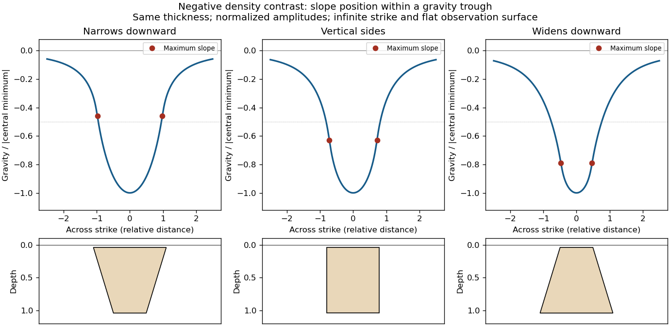
This qualitative inference assumes approximately comparable simple bodies, uniform geophysical density contrast, and a properly removed regional field. Gravity inversion is non-unique: lateral density changes, multiple bodies, and a buried top can imitate changes of wall slope. Use the seismic reflection constraints to test the interpretation.

Let $S_g$ be the fraction of the pore space occupied by gas, and let $\varphi$ be the porosity. At fixed porosity and unchanged rock framework, the bulk density isReplacing water with much less dense gas therefore decreases the bulk density approximately linearly, as in Figure 1. The liquid and gas densities here are those at reservoir conditions.

A pore fluid has negligible static shear modulus, so the rock framework chiefly controls the effective shear modulus $\mu$. If $\mu$ changes little, $V_s=\sqrt{\mu /\rho }$ increases gently as the density falls. This does not imply that S waves travel through the pore gas itself: their restoring force comes from the connected solid framework.

The P wave speed depends on both bulk modulus and shear modulus:Gas is much more compressible than water. Even a small connected gas fraction can strongly reduce the effective fluid bulk modulus, approximately through the compliance average ${\kappa }_f^{-1}\simeq (1-S_g)/{\kappa }_w+S_g/{\kappa }_g$ for a pressure-equilibrated mixture. The saturated rock's effective bulk modulus consequently falls rapidly at first, overwhelming the smaller density reduction and causing the sharp initial fall in $V_p$. Once the fluid is already very compliant, further gas replacement changes the stiffness less; the continuing density decrease can then make $V_p$ rise again. Figure 1 assumes a particular saturation response: patchy fluids, changing effective pressure, and frequency-dependent fluid motion can alter it. The plotted $V_s$ is only nearly constant, so the plot should not be interpreted as an exact fixed-$\mu$ constitutive model.

For incidence from cap rock (1) into reservoir (2), use the conventional normal-incidence stress-amplitude reflection coefficientHere acoustic impedance is the P wave impedance; $\rho V_s$ is the corresponding shear-wave impedance. Positive $R$ preserves the chosen stress-wave seismic reflection polarity; negative $R$ reverses it. These are amplitude coefficients, not reflected energy fractions. At normal incidence in the ideal isotropic model there is no P-to-S mode conversion. The cap-rock impedances are

The following are approximate readings of the supplied Figure 1 PNG, checked against the matching source PDF, rather than exact tabulated parameters. At zero gas, use $\rho \simeq 1.75\mathrm{g}\mathrm{c}{\mathrm{m}}^{-3}$, $V_p\simeq 1.75\mathrm{km}{\mathrm{s}}^{-1}$, and $V_s\simeq 0.60\mathrm{km}{\mathrm{s}}^{-1}$; at full gas use $\rho \simeq 1.25\mathrm{g}\mathrm{c}{\mathrm{m}}^{-3}$, $V_p\simeq 1.15\mathrm{km}{\mathrm{s}}^{-1}$, and $V_s\simeq 0.65\mathrm{km}{\mathrm{s}}^{-1}$. The left-hand $V_p$ endpoint is crowded against the axis and the density curve; readings differing by roughly $0.05$ in the plotted units are reasonable. The resulting coefficients deserve about two significant figures, not the apparent precision of the intermediate arithmetic.

Both end members change seismic reflection polarity, but the P wave change is much larger: approximately $+0.15$ to $-0.22$, compared with $+0.08$ to $-0.05$ for S waves. Thus a calibrated P wave survey is better for distinguishing these two saturation end members and should give a stronger reflection from the fully gas-filled reservoir. A negative P wave reflection relative to the water-filled prediction is a useful gas indicator in this stipulated model. In a real seismic reflection survey, lithology, porosity, effective pressure, and seismic wavelet phase also affect the response, so a bright or reversed reflection alone does not prove the presence of gas.

For the fully water-filled reservoir, the approximate densities and wave speeds giveand henceBoth are positive: the reservoir has larger P wave and shear-wave impedances than the cap rock, and neither reflection reverses the chosen stress-wave seismic reflection polarity.

taphonomic bias is systematic distortion of biological information between a living community and the fossil record. Death, carcass decay, scavenging, transport, burial, chemical alteration, exposure and collection all filter what is observed. A deposit therefore samples organisms, body parts and environments unequally. This is more than incompleteness: preferential preservation of a particular tissue or habitat can produce a misleading pattern of abundance, anatomy or evolutionary timing.

An autochthonous fossil assemblage contains remains preserved where the organisms lived; an allochthonous fossil assemblage contains material transported from elsewhere. These describe provenance, rather than two levels of fidelity. In an allochthonous fossil assemblage, currents can separate elements by size, shape and density, concentrate resistant teeth or scales, remove delicate bodies and mix organisms from different habitats. Erosion and redeposition can also introduce older fossils into younger sediment. Such reworking differs from simple transport of recently dead animals. time averaging mixes deaths from different times even without long-distance transport. A concentration of robust remains consequently need not represent either a locally abundant living population or a single ecological event.

An autochthonous fossil assemblage avoids some transport distortion, but still selects organisms and characters. A bottom-dwelling community rapidly buried in place can be unusually well represented while swimmers above it, unmineralized tissues and organisms living outside that depositional setting are missing. Conversely, an intact carcass can travel before burial, whereas locally decayed remains can become disarticulated without transport. Articulation, abrasion, preferred orientation, sedimentary context and age agreement must therefore be evaluated together. Local preservation does not imply an unbiased biological census.

The contrast between cyclostomes and early members of the gnathostome lineage is particularly revealing. Living cyclostomes, hagfish and lampreys, have no extensive mineralized external skeleton comparable to the armour of many early jawless relatives of gnathostomes. Their bodies are dominated by tissues whose preservation usually requires exceptional conditions. The abundance of isolated mineralized scales, plates or teeth can thus make a hard-bodied lineage conspicuous where a soft-bodied contemporary is virtually invisible. Importantly, the armoured jawless assemblage traditionally called ostracoderms is not simply the ancestral cyclostome record: many of its members belong on the gnathostome stem. Absence of jaws does not by itself establish cyclostome affinity.

There is also a character-level filter. Robert S. Sansom and colleagues followed experimental carcass decay of living chordates, and then examined hagfish and lampreys in detail. Anatomical characters did not disappear at random: loss of diagnostic features could make a derived animal appear more primitive. This produces stemward slippage if investigators mistake an unpreserved feature for a feature absent in life. The result is relevant both to isolated soft-bodied fossils and to the apparently long primitive intervals preceding well-preserved groups.^[ref][ref]

A useful experimental design records fresh anatomy first, samples replicated carcasses through time under stated temperature and chemical conditions, and scores the same characters in each specimen. Comparisons between animals and between preservational conditions test whether the loss order is reproducible. Such experiments identify plausible biases; they do not recreate every burial chemistry or prove that every uncertain fossil has undergone the same sequence. In a phylogenetic character matrix, genuinely unobservable anatomy should normally be coded as unknown rather than automatically absent. Comparison across differently preserved specimens can sometimes recover information that one specimen lacks.

Exceptional discoveries show what the ordinary record omits. The Late Devonian lamprey Priscomyzon from South Africa preserves a recognizable oral apparatus and branchial region without a massive mineralized skeleton. It shows that early lamprey anatomy can be recovered when the appropriate soft-tissue window is available; the gap before such a discovery is not evidence that the lineage had just originated.^[ref] The Cretaceous hagfish Tethymyxine preserves evidence including slime-producing structures, allowing characters unavailable in most older deposits to be brought into an analysis using phylogenetics. It supplies a minimum occurrence and anatomical information, not the date when hagfish originated.^[ref] Conversely, Early Silurian Qianodus is known through mineralized tooth whorls: such durable small remains can establish an early occurrence of a toothed gnathostome even where complete bodies are missing.^[ref]

The defensible comparison concerns preservation probabilities as well as biological histories. First fossil occurrences are minimum ages, and unequal counts need not measure unequal diversity. Independent anatomical characters, comparable depositional settings, searches for small hard parts and exceptional soft-tissue deposits together give a better test of early vertebrate history than a literal reading of the most conspicuous remains.

A colloidal grain in a liquid is large enough to see with a microscope, yet small enough for thermal motion to compete with its tendency to settle. In the Perrin sedimentation experiment, the equilibrium number density falls with height: a visible miniature atmosphere. Counting grains at different heights measures an energy scale; tracking their Brownian motion measures a transport rate. Connecting both to the same Avogadro constant makes the experiment a quantitative test of kinetic theory. The Wiener measure describes an idealized path law; these measurements instead test a physical model and its material parameters.

Jean Baptiste Perrin's 1909 memoir traces his sedimentation experiments to May 1908. It reports relative counts $100$, $47$, $22.6$, $12$ at heights $5$, $35$, $65$, $95\mu \mathrm{m}$, and compares radius estimates from Stokes settling velocity, counted grain mass, and rows of touching grains.^[ref]

The 1926 lecture describes resin precipitated from alcohol into water, washed and fractionated by centrifugation to obtain nearly monodisperse gamboge or mastic grains. Diameter and density were measured separately. A sealed slide-and-cover-glass chamber prevented evaporation; a vertical microscope resolved roughly $2\mu \mathrm{m}$ layers through a roughly $0.1\mathrm{mm}$ depth. Refocusing and photographing compared layer populations after equilibrium; changing temperature reversibly changed the distribution.^[ref]

In Les Atomes (1913), Jean Baptiste Perrin restricts the eyepiece view to fewer than five or six grains and alternates observations between heights. Focus displacement requires a refractive index correction to recover actual layer separation. Horizontal positions were marked with a camera lucida, usually every $30\mathrm{s}$, and distances calibrated with a micrometer; the polygon joins sampled positions rather than recording the intervening trajectory.^[ref][ref]

A galaxy cluster whose X-ray-emitting core is a well-studied example of interaction between radio bubbles and cooling gas. density fronts and ripples provide diagnostics of the mechanical energy released by the central active galaxy.^[ref]

A driver excites charge-density oscillations in a plasma whose longitudinal electric field transfers energy to a trailing witness beam. Density fixes a characteristic plasma frequency and wavelength, while driver shape and loading determine the actual field and transfer efficiency.

A pendulum of length $L$ in vertical gravity $g$ is weakly attracted horizontally by an added long circular cylinder of line density $\lambda$. Outside it, $g_h=2G\lambda /r$ at axis distance $r$. Small-angle equilibrium gives horizontal deflection $d\simeq L{g}_h/g=2GL\lambda /(rg)$. Removing the cylinder's mass reverses the change. It is a before/after differential estimate; finite length, a nonhorizontal radial direction and mechanical motion require corrections.

A charge cloud $\rho =A/r$ for $0<r<a$ encloses $Q(r)=2\pi A{r}^2$. With no central point charge and potential zero at infinity, Gauss's law gives $\varphi =A(2a-r)/(2{ϵ}_0)$ inside and $A{a}^2/(2{ϵ}_{0}r)$ outside. The density singularity is integrable, and the potential is finite at the origin.

A local compensation model in which columns of different density reach a common compensation depth. Higher surface topography is associated with a less dense column; density variation replaces the variable-root mechanism of an Airy model.

A one-dimensional reference model combining elastic wave speeds, density and attenuation, developed by Adam M. Dziewonski and Don L. Anderson. It incorporates joint seismic and global integral constraints rather than treating density as a direct travel-time measurement.

For $p=a_T^2\rho$, spherical hydrostatic equilibrium admits $\rho =a_T^2/(2\pi G{r}^2)$ with $M(r)=2a_T^{2}r/G$. Matching an external pressure $p_0$ fixes $r_s=a_T^2/\sqrt{2\pi G{p}_0}$. The central density is singular although the enclosed mass tends to zero; this is one branch, not every finite-centred isothermal cloud.