Hydrostatic balance and the ideal gas law give , hence approximately with for weak temperature variation. For well-mixed absorber abundance, , while pressure broadening gives . Thus and its integral above height has the same scale. Therefore
The factor two depends on both pressure dependence of absorption and constant mixing ratio; it is not the ordinary density scale height.
A dynamical collapse law specifies stochastic changes of the wavefunction, including a rate, localization scale and probabilities. Such changes can suppress macroscopic superpositions, but a law for a mathematical state does not automatically identify the stuff composing a macroscopic table. If the wavefunction is on configuration space, one must still explain how it represents a three-dimensional distribution of matter and records.
One option defines mass density in ordinary space by . A localization then changes this density so that a single dominant macroscopic pattern remains. The formula is additional interpretive structure, even if it introduces no independent evolving variable beyond the wavefunction. Another option takes discrete spacetime localization events as the primitive ontology. These two proposals can accompany closely related wavefunction dynamics while telling different stories about what matter is.
This is why mass density in particular is not logically mandatory, but some account of the relation between collapse and ordinary physical objects is required if the theory is offered as a complete ontology. A wavefunction-only view may argue that no further primitive stuff is necessary, yet it owes an explanation of spatial localization and records on that basis. Merely asserting that interference terms become small is not that explanation.
Additional posits can also have costs: small wavefunction tails survive finite localization, and the ontology must say what their tiny matter components or corresponding events mean. Choosing primitive ontology and handling such tails are distinct from specifying the stochastic dynamical law. A defensible collapse interpretation therefore makes both commitments explicit rather than suggesting that adding randomness alone solves every part of the measurement problem.[ref][ref]
Hamilton's equations define phase-space velocity . Its divergence is
Thus infinitesimal phase-space volumes are preserved, assuming sufficient differentiability. This is Liouville's theorem; spatial density alone need not be incompressible because the statement concerns the combined coordinate-momentum space.
Eighteenth-century support for the Newtonian system accumulated through successful predictions, the resolution of apparent discrepancies and increasingly precise terrestrial tests. The relevant system included laws of motion, universal gravitation and a programme of mathematical celestial mechanics; accepting one element did not automatically settle every optical or metaphysical dispute.
Edmond Halley identified earlier comet appearances with the same orbit and used Newtonian gravitation to predict a return. Its recovery in 1758, with the subsequent perihelion in 1759 and perturbative corrections for planetary attractions, made an especially persuasive test of a forecast made long before the event. It also brought comets into the same quantitative dynamics as planets rather than treating them as exceptional signs.[ref]
Geodetic expeditions compared meridian arcs at different latitudes. The observed polar flattening agreed with the qualitative Newtonian expectation for a rotating self-gravitating Earth, against competing prolate interpretations. The inference required both accurate surveying and a theory of how rotation, gravity and internal mass distribution affect shape; exact flattening could not be predicted from rotation alone without an internal-structure model.[ref]
Lunar and planetary perturbation theory provided a sustained, more demanding test than unperturbed Keplerian ellipses. Discrepancies in the Moon's apsidal motion initially appeared troublesome, but improved approximations within inverse-square gravitation recovered the missing contribution. Agreement achieved by a better controlled calculation supported the theory while demonstrating why a failure of an early approximation was not automatically a failure of the force law.
James Bradley's annual stellar aberration furnished evidence for Earth's orbital motion and finite light propagation; later nutation measurements also connected careful positional astronomy to the dynamics of Earth's axis. Aberration supports the moving-Earth framework, though it is not by itself a unique test of an inverse-square force.[ref]
Finally, Henry Cavendish's torsion-balance experiment in 1798 measured attraction between laboratory masses and inferred Earth's mean density. It extended gravitation from celestial fitting to a quantitatively controlled terrestrial attraction; describing the original aim as determining Earth's density is historically more accurate than saying he set out to measure a modern separately defined . Together these tests supplied converging support across scales. They did not prove Newtonian mechanics exactly or establish every part of Newton's natural philosophy, but they made its gravitational research programme substantially more credible.
Assume a dilute nondegenerate hydrogen gas in thermal and chemical equilibrium, with Maxwell-Boltzmann translational partition functions, ground-state neutral atoms, single ionization and charge neutrality . For , chemical equilibrium gives . The ideal-gas relation , with , gives
Neglecting the electron mass in and using the ground-state electronic statistical weights, and with cancelling nuclear-spin factors, this becomes
Excited neutral states have an energy gap of at least above the ground state. At the temperatures relevant to the plotted maximum their Boltzmann factors are very small despite the finite degeneracy increase. Highly excited levels also require a physical plasma cutoff; the untruncated infinite isolated-atom partition sum is not a valid finite-density model. Ground-state dominance is an approximation in this regime, not a theorem at all temperatures.
Take the heating process to keep the total hydrogen-nucleus density fixed, so . This fixed-density assumption is needed to determine from the curve; freely expanding gas would require its density history. The excited-to-ground ratio is . Therefore
At low temperature excitation is suppressed. At higher temperature excitation grows, but eventually ionization removes neutral atoms and the excited-neutral abundance decreases. To locate the maximum quantitatively, write . From ,
Setting gives
Reading the original graph gives K and . With eV, this implies and . Substitution into
gives approximately . The result is particularly temperature-sensitive because of the Saha exponential; using K gives about , while the coarse K reading gives about . The plotted height is consistent with this range and should not be used to claim more precision than the source graph provides.
The plasma parameter is the mean number of electrons in a Debye sphere. With electron Debye length ,
Large describes weakly coupled collective screening; a single electron does not dominate its screening cloud. For a small uniform electron displacement relative to fixed ions, the restoring field gives , hence
This cold-electron oscillation estimate neglects thermal dispersion and ion motion.
Using the stipulated collision-time approximation,
With and , the kinetic estimate gives
The elementary single-speed estimate corresponds to ; velocity averaging and the stated collision model are represented by the supplied . A detailed Coulomb transport calculation also contains a Coulomb logarithm and cannot be inferred precisely from this simplified expression.
The electron thermal energy density is . Transporting all of it at the thermal speed gives the free-streaming scale
For heat flowing in the positive direction, . Inserting into gives
This flux-limiting criterion expresses the failure of a local diffusive description when an electron samples a substantial change in temperature over a transport path.
For the stipulated carbon plasma and , setting the gradient equal to gives a critical flux fraction of order . Fourier transport is invalid according to this test when ; a still larger actual gradient raises the critical value. Thus the source's request for a minimum has the inequality reversed: the calculation gives an upper threshold, not a positive minimum. An arbitrarily smaller positive makes the criterion easier to satisfy. The exact numerical threshold is evaluated in the independent check.
Use positive angular frequencies and abbreviate , . The left-handed index is . It is negative below its positive zero,
For the right-handed mode, . Below the cyclotron resonance its denominator is negative and the index square is positive. Just above the resonance it is negative until
This is the lossless electron-only cold-plasma model. Ions, collisions and resonance absorption matter outside its applicable range.
For a whistler with and ,
The travel time through a uniform slab is . In terms of ordinary frequency,
An arbitrary emission time changes the intercept, not the slope. The original figure labels a dispersion constant : it is the reciprocal of the plotted slope, not the slope itself. Therefore
For nT and m this gives , , and
The resulting forbidden right-handed frequency width is
The lower edge is about kHz and the upper edge about kHz. In the real nonuniform plasma, the travel-time coefficient measures a path integral proportional to . The inferred density is consequently an effective uniform-slab estimate, not a unique local density at the spacecraft. Uncertainty in the path and magnetic field likely exceeds the formal error in .
The mean witness gradient must be . To turn this into a density estimate, assume an accelerating wake amplitude of order the cold plasma wave-breaking scale,
Eliminating gives
The associated plasma wavelength is about micrometres, illustrating why a short driver structure is required. The given length and energy gain do not uniquely fix density without an assumption about wake amplitude relative to the plasma scale. Driver shape, beam loading, relativistic wave-breaking corrections and matching to a Positron witness are substantive additional issues; the estimate is a scale calculation, not a completed accelerator design.
A thin spherical shell of thickness has mass . Balancing its inward gravitational force with the pressure difference across its faces gives
For a transparent estimate take constant density and negligible surface pressure. Then , so integration gives
Combining with the ideal gas law and yields K. The less specific virial scaling gives K.
The real Sun is strongly centrally concentrated: a uniform-density model substantially underestimates central pressure and is not a detailed solar model. Its value is a justified scale estimate, while more realistic structure produces central temperatures of order K and central pressures of order Pa. Hydrostatic equilibrium alone does not uniquely determine both profiles without an equation of state and a density/thermal model.
The radiation pressure at a photospheric temperature near K is only about Pa. For an illustrative photospheric gas density and mean molecular weight near , the ideal gas pressure is about Pa. Thus gas pressure dominates those outer layers by many orders of magnitude. Both the temperature and density are needed: low temperature alone is not a complete comparison.
For homologous stars, hydrostatic and ideal-gas estimates give and . Therefore
with a structural coefficient independent of mass only under the homology assumption. As mass rises, radiation becomes increasingly important. A rough solar interior normalization of - suggests equality after a mass increase by tens, while realistic radiation-dominated structure and composition shift the scale; stars of order are a useful estimate for strong radiation support. The very small photospheric ratio must not be used as a universal normalization for their whole interiors.
Radiation also transfers outward momentum. Comparing radiative acceleration with gravity gives the Eddington luminosity
Near this scale, radiatively driven winds and envelope instabilities can remove matter or impede further accretion. Opacity, composition, rotation, mass loss and formation history affect the limiting stellar mass. The Eddington condition is a luminosity-to-mass constraint, not a unique composition-independent maximum stellar mass.
Opacity is the extinction cross section per unit mass for radiation; a frequency-dependent value gives when emission is considered separately. Stellar radiative diffusion generally uses an appropriately weighted Rosseland mean opacity. The associated local mean free path is of order .
At sufficiently high temperature the material is highly ionized, and scattering by free electrons is often dominant for ordinary stellar densities and photon energies well below the electron rest energy. Bound-bound and bound-free absorption weaken as bound electrons disappear; free-free absorption can still matter depending on temperature and density. Thus “high temperature” does not fix the dominant opacity at every possible density. The next part explicitly imposes a Kramers absorption law as a separate scaling model.
Use characteristic stellar values in the supplied radiative temperature gradient: . Hence . With Kramers opacity, ,
Hydrostatic support by an ideal gas gives , or . Substitution then yields
The result assumes homologous density and temperature profiles, comparable structural constants, gas-pressure support and radiative transport throughout. It is not simultaneously an electron-scattering-opacity result; replacing Kramers opacity changes the exponents. Convection, degenerate cores or a different opacity regime limit quantitative application to real evolved helium stars.
The integrated spectrum combines stars moving toward and away from us within the galaxy, broadening their absorption by Doppler shifts. Assuming instrumental and individual-stellar widths have been removed or are negligible, the line-of-sight velocity dispersion is
The angular half-light radius at the low-redshift distance is kpc. For a pressure-supported, approximately isotropic equilibrium spheroid with a standard structural virial coefficient of order five, use
The coefficient represents assumed density profile, aperture and orbital structure; a different reasonable mass estimator changes the result by an order-unity factor. Treating as a luminosity distance and using would reduce the radius and mass by about four percent here.
The distance modulus is about . The magnitude within therefore corresponds to and
Doubling the half-light luminosity gives
This ratio is compatible with an old stellar population plus possible dark matter. It is larger than a solar-like mass-to-light ratio, but does not by itself isolate a unique dark-matter fraction: stellar age, initial mass function, anisotropy and the virial coefficient are not specified. Counting the quoted half-light magnitude as the total would incorrectly double the inferred ratio.
Hydrostatic equilibrium means that the local pressure gradient balances gravity, with no large acceleration or strength-supported departure from that balance. In a spherical planet,
Here is the enclosed mass, not a constant total mass at every interior radius. If composition is uniform and the radial thermodynamic path is adiabatic, the relevant bulk modulus is . The chain rule then gives the Adams-Williamson relation
A phase transition or composition jump must be treated separately; its density change is not obtained by integrating one smooth homogeneous-adiabatic equation through it.
The seismic parameter is
The shear modulus measures resistance to shear deformation. Solids with transmit shear waves; an ideal fluid has zero static shear modulus, so it cannot carry a bulk S wave, while compressional P waves can still propagate through its nonzero bulk modulus.
Limitations include uncertain seismic coverage, temperature and composition tradeoffs, nonadiabatic boundary layers, phase changes, lateral heterogeneity, rotation and finite material strength. Small asteroids and comet nuclei commonly retain irregular shapes because their self-gravity is too weak to overcome strength and impact history; a few larger bodies, such as Ceres, are much closer to global hydrostatic figures. A spherical shape alone is not a complete proof of present hydrostatic equilibrium.
Two complementary remote constraints are precise spacecraft tracking, which measures gravitational harmonics and constrains mass distribution when combined with shape and rotation; and tidal or rotational measurements, such as Love numbers, librations and spin precession, which constrain deformability, moment of inertia and possible fluid layers. Magnetic induction measurements in a time-varying external field can provide an additional conductivity constraint, but are not a unique density inversion.
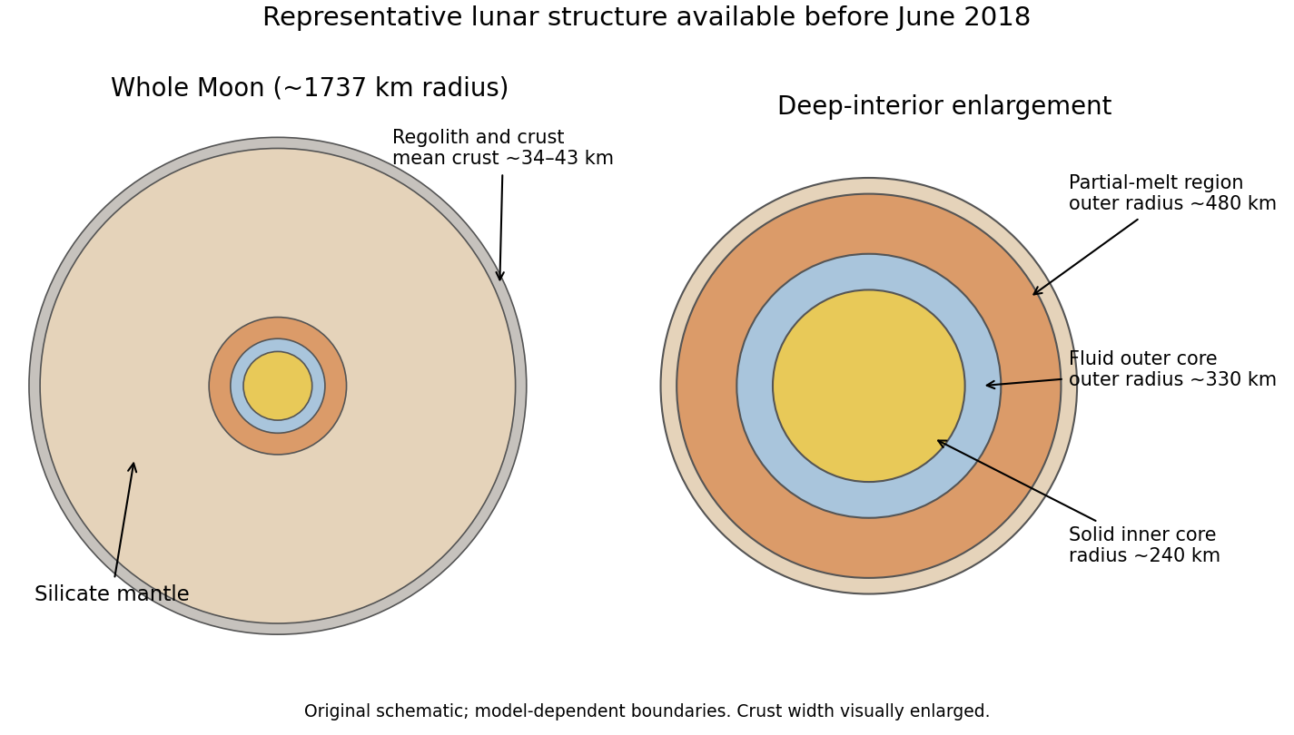
For the June 2018 lunar picture, start with a regolith and fractured crust, a largely anorthositic crust tens of kilometres thick, a silicate mantle, a deep partially molten region and a small iron-rich core. GRAIL and Apollo-based models gave a global mean crustal thickness around - km.[ref] A representative seismic model has a partial-melt boundary near radius km, a liquid outer-core boundary near km and a solid inner-core radius near km; these are model-dependent radii from the centre, not depths below the surface.[ref]
Figure 1.
A representative pre-June-2018 lunar interior model
. An original schematic cross-section labels the crust, silicate mantle, deep partial-melt region, fluid outer core and solid inner core. Approximate central layer radii are 480, 330 and 240 kilometres; the thin crust is shown with a visually enlarged width and all boundaries are model dependent. Details.
The long-running Apollo network had only four principal stations on the near side, with poor global coverage and strong scattering in the fractured near-surface material. Far-side structure and weak deep reflected phases were therefore difficult to constrain. The historical date matters: the answer does not import later Mars seismology or later lunar-core refinements into the 2018 premise.
Set with the convention of part b. Then
Thus ordinary solid-state temperatures are far below this rough overlap scale. The electrons need quantum statistics and quantum states throughout that regime. The number is an order-of-magnitude wavelength criterion, not an exact Fermi temperature: electron density, electronic band structure, effective mass and the numerical convention all matter.
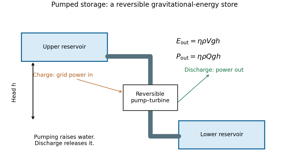
A pumped-storage plant moves water uphill using electrical power, then returns it through a turbine and generator when electricity is needed. The upper and lower reservoirs set the usable volume and head; pumps, penstocks, valves and reversible pump-turbines set the power and flow. The plant stores energy rather than generating net energy over a cycle.
Figure 1.
Gravitational storage separates reservoir energy capacity from pump and turbine power
. An original functional diagram shows an upper and a lower reservoir connected through a penstock and reversible pump-turbine. Charging uses grid electricity to lift water; discharge returns gravitational potential energy through the generator. Details.
For constant head, the gravitational energy is . With the stated generation efficiency,
At GW, gives
Head variation, dead volume and hydraulic losses beyond the stipulated efficiency have been neglected.
To deliver kWh with the same head and efficiency needs of water, roughly a m cube, together with a m elevation difference and a lower reservoir. At a m head it would need about . This contrasts with the small fuel volume: the useful energy density of lifted water depends on its external head, not its chemical composition.
Pumped storage offers long service life, fast dispatch, substantial power, and separate choices of storage volume and turbine rating. Its drawbacks include geographic constraints, construction cost and time, ecological impacts, evaporation and water requirements, plus round-trip losses. The quoted generation efficiency alone is not the round-trip efficiency because pumping also consumes more than the stored potential energy.
The rock cylinder has mass and rises through . Equating its useful energy to the reservoir result cancels the common efficiency and gravity:
Its height is about m and its lift about m, ignoring buoyancy as instructed. Stored energy scales as , excavated volume roughly as , and lined area as . If excavation dominates cost, cost per unit stored energy decreases approximately as . Seals, increasing pressure, geology, leakage, supporting structure and power equipment can change that scaling; a volume law is not a complete cost model.
The coil-globule transition is the contraction of an isolated flexible polymer as solvent quality worsens. A swollen chain in a good solvent has size in the Flory approximation. At the theta temperature the effective two-segment excluded volume vanishes and . A poor solvent favors a dense polymer globule, with at fixed internal density.
The competition is visible in the scaling free energy
For , elastic cost balances two-segment repulsion to give the swollen-coil law. At , three-segment repulsion stabilizes ideal-chain scaling; for , attraction balanced by the positive three-segment term gives . The dense polymer globule also has an interfacial free energy. The scaling expression explains regimes, not all fluctuation corrections or a detailed finite-chain transition curve. A finite chain crosses over smoothly; the sharp theta-point limit refers to indefinitely long chains.
A dilute-solution light-scattering experiment can follow radius of gyration while changing temperature or solvent composition. Measure at several concentrations and extrapolate toward isolated chains; check molecular-weight distribution, reversibility and the absence of growing multi-chain aggregates. dynamic light scattering measures hydrodynamic size, which is related to but distinct from radius of gyration. A falling scattering-derived size accompanied by a rising aggregate population cannot by itself establish single-chain collapse. solvent quality controls conformation through the balance of segment interactions and conformational entropy.
Balancing buoyant weight with Stokes drag gives
This needs isolated spherical particles, low Reynolds number and negligible wall corrections. The supplied settling measurement gives , hence . Its Reynolds number is about , consistent with the approximation.
Compare gravitational work over one radius with thermal energy, or use with . The gravitational Peclet number gives
Below this sedimentation-Brownian crossover radius Brownian motion dominates settling on the particle-size scale. It does not eliminate gravity: the sedimentation scale height is . For negligible concentration gradients across a sample height , the stronger condition is . No universal permanently nonsedimenting size follows without a length/time criterion.
Brownian encounters bring small particles into contact; van der Waals attraction can then bind them. Surface charge can create a repulsive barrier through Debye screening of colloid repulsion. For a monovalent salt reservoir with number density of each ionic species, Poisson–Boltzmann theory has
For , linearization gives , with . If instead means total ion density, the factor two is absent. The planar potential decays as ; a sphere has an additional factor. This mean-field approximation neglects specific adsorption, ion correlations and finite ion size.
DLVO theory adds screened repulsion to dispersion attraction. At small surface separation for equal spheres of radius , a useful schematic form is
with a short-range repulsive core needed outside the continuum model. Low salt can leave a barrier many times , giving kinetic stability. Higher salt shortens the repulsion and can lower or remove the barrier, allowing coagulation into a deep primary minimum. The primary and secondary DLVO minima have different consequences: a shallow secondary minimum permits looser, sometimes reversible aggregation. The surface boundary condition affects ; screening length alone is not a complete measured interaction law. Non-DLVO hydration or steric forces can matter at contact.
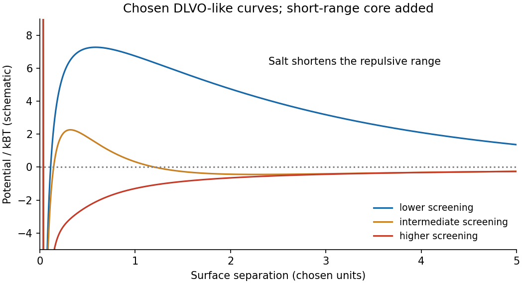
Figure 1.
Original schematic DLVO potentials showing barrier reduction with increased screening
. Details.
For a long ideal chain of statistical segments of length , . At fixed repeat chemistry and statistical segment length, molar mass is proportional to . The molecular-weight scaling of an ideal-chain gyration radius thus gives
The supplied size and ideal statistics are used as stipulated; an independently tabulated coil size would not replace the given baseline.
solvent quality changes the balance of segment–segment and segment–solvent contacts. In a good solvent, excluded-volume repulsion swells a sufficiently long isolated chain, with , in three dimensions; the Flory approximation gives . At theta conditions the effective two-segment excluded volume vanishes and the ideal exponent is recovered for long chains. A poor solvent favors a compact polymer globule, whose large-chain size scales approximately as at fixed internal density. solvent and temperature can also change local persistence length and hence the prefactor. These different conformations need not have the same radius at the same molar mass.
polymers at interfaces balance favorable surface contacts against lost conformational entropy and interactions among neighboring chains. At an attractive solid–liquid interface, an adsorbed polymer train consists of consecutive bound segments. An adsorbed polymer loop leaves the surface and returns to it, while an adsorbed polymer tail extends to a free chain end. A chain can contain all three, so adsorption does not imply a completely flattened molecule. Surface affinity, solvent quality, persistence length, chain length and concentration control the balance and the resulting segment-density profile.
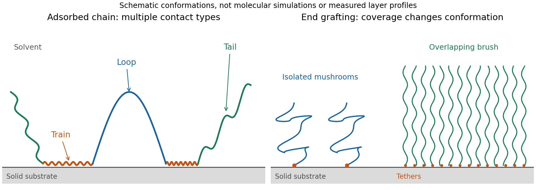
Figure 1.
Original schematic of adsorbed trains, loops and tails, and the crossover from isolated grafted mushrooms to an overlapping polymer brush
. Details.
adsorption gains energy of order per bound segment but reduces the number of accessible chain configurations. Weak adsorption can be described through adsorption blobs whose thickness exceeds the statistical segment length; each blob loses an energy of order through confinement. Stronger attraction generally creates more contacts and a more compact layer, while loops and tails can still dominate its outer extent. A measurement of adsorbed mass alone therefore does not determine layer thickness or conformation.
End-grafted chains are different: their attachment is fixed at one end. At grafting density , the mean lateral spacing is . At low coverage the chains behave as isolated polymer mushrooms. The polymer mushroom-to-brush crossover occurs when . At higher coverage in a good solvent, crowding makes chains extend away from the surface. A free-energy balance per chain,
combines stretching entropy with repulsive excluded volume . Minimization gives , or
This is a scaling result with an undetermined order-one coefficient, valid for overlapping chains stretched below their contour length. In a compact poor-solvent layer, a roughly fixed internal polymer volume fraction instead gives .
Small-angle neutron scattering on end-grafted polydimethylsiloxane layers on porous silica has distinguished the good- and poor-solvent density exponents. The chemical system and scattering contrast matter: changing solvent quality should be separated from changing graft coverage, chain molar mass or adsorption strength.[ref]
An interface can also localize chains of a block copolymer when its blocks prefer different media. Such layers change interfacial tension and can stabilize dispersed droplets or particles through steric repulsion. Overlapping layers in a good solvent cost osmotic and conformational free energy; incomplete adsorption can instead produce polymer bridging between particles. Nonadsorbing chains can cause depletion attraction. Thus the presence of a polymer does not by itself guarantee stabilization.