Anatomy

Sampling limits in anatomical variant frequencies distinguish how often a structure was observed in a specimen set from how common it is in a defined population. The denominator must identify the independent anatomical unit: people, hearts, limbs or images are different units. Preserved material and the detection procedure also determine what can be observed.

A primary example dissected 37 formalin-fixed adult human hearts, finding the small cardiac vein in 54% of specimens and an approximately 1 mm venous connection in 19%.^[ref] Those percentages describe that study's material; they do not establish a universal frequency across populations or measurement methods.

Under an original independent, representative-sampling model with perfect detection, a binomial distribution gives

X \sim Bin (n, p)

. If no examples of a specified variant are seen,

Pr (X = 0) = (1 - p)^{n}

. Inverting the one-sided test at level

α

gives

p_{upper} = 1 - α^{1/ n} .

For a hypothetical zero observations among 37 specimens and

α = 0.05

, the upper limit is approximately 0.0778, not zero. The familiar approximation

- lo g (α) / n

is about 0.0810 here. These are illustrations, not unreported results from the anatomical paper.

Detection-limited anatomical prevalence bounds add another assumption explicitly. If a real variant is detected with probability

q

and false detections are absent, the observed-event probability is

qp

. Zero observed cases therefore gives

p_{upper} = min {1, (1 - α^{1/ n}) / q}

when

q

is known. At stipulated

q = 0.5

, the example limit becomes approximately 0.156. Unknown detection probability cannot be repaired by reporting a more precise count.

Repeated photographs of the same heart do not create independent new hearts. Counting every image as an independent specimen would artificially narrow a confidence interval. Selection of unusually accessible, preserved or clinically referred specimens can also produce bias that a binomial distribution does not quantify. A useful anatomical report states selection, preservation, observation criteria and the denominator alongside its frequency; uncertainty calculations then make their sampling and detection assumptions visible.

Detection-limited anatomical prevalence bounds

Detection-limited anatomical prevalence bounds account for the fact that a structure can exist without being recognized by the observation method. Zero observed variants constrain the probability of observing a variant; translating that into a population frequency requires a detection model. In anatomical research, specimen preservation, resolution and the definition of a positive observation belong to that model.

A primary coronary-venous study dissected 37 formalin-fixed hearts and reported frequencies of visible venous structures.^[ref] Its specimen count is a concrete setting for explaining sampling, but the detection probabilities below are hypothetical, not estimates from that paper.

Let

p

be population prevalence and

q

the probability of detecting a present variant, with no false detections. For independent specimens, the observed count has a binomial distribution with event probability

r = qp

. Zero detections among

n

gives the one-sided upper bound

r_{U} = 1 - α^{1/ n}, p_{U} = min {1, r_{U} / q} .

Joint coverage in detection-calibrated prevalence bounds matters when

n = 37

α = 0.05

and known

q = 0.5

, this gives

p_{U} \approx 0.156

. The confidence statement depends on

q

being known, not merely on a convenient assumed value.

q

is estimated. Suppose a calibration gives a lower bound

q_{L} > 0

with coverage at least

1 - β

, while

r_{U}

has coverage at least

1 - α

. Whenever both bounds cover,

p \leq r_{U} / q_{L}

; the union bound guarantees combined coverage at least

1 - α - β

, without requiring independence of the two bounds. Allocating

α = β = 0.025

and stipulating a calibrated lower bound

q_{L} = 0.5

gives

p_{U} \approx 0.190

for the same zero count.

False detections change the relation to

r = f + (q - f) p

, where

f

is the false-detection probability for absent structures. If

q = f

, the observed frequency carries no information about prevalence. Simply dividing by

q

is then invalid. Detection controls should therefore distinguish missed structures from false recognitions.

These bounds do not repair unrepresentative specimen selection or treating repeated images as independent bodies. Report the anatomical unit, detection validation and target population alongside a confidence interval; more decimal places cannot substitute for those assumptions.

Joint coverage in detection-calibrated prevalence bounds

Joint coverage in detection-calibrated prevalence bounds controls the chance that both the observed-event bound and its detection calibration are valid. A prevalence calculation that substitutes an estimated detection probability into a sampling bound does not automatically retain the original confidence level.

In an original model with no false detections, prevalence

p

and detection probability

q > 0

give observed-event probability

r = qp

. Let

r_{U}

be an upper confidence bound with coverage at least

1 - α

, and

q_{L} > 0

a lower confidence bound with coverage at least

1 - β

. On the event that both bounds cover,

p = \frac{r}{q} \leq \frac{r _{U}}{q _{L}} .

The union bound gives

Pr (r > r_{U} or q < q_{L}) \leq α + β

. Hence

p_{U} = min {1, r_{U} / q_{L}}

has coverage at least

1 - α - β

. This argument does not require independence between the two estimates, but it does require valid marginal bounds for the stated model. If no positive lower bound on

q

is established, the resulting prevalence bound may be uninformative.

Exact extreme-count examples follow by inverting binomial distribution probabilities. NIST describes exact interval construction from binomial tails and distinguishes one-sided limits.^[ref] Zero detections among

n

specimens gives

r_{U} = 1 - α^{1/ n}

. Detecting all

m

independently known positive calibration specimens gives

q_{L} = β^{1/ m}

. These are one-sided extreme-case formulas derived from

(1 - r)^{n}

and

q^{m}

For stipulated

n = 37

m = 20

and

α = β = 0.025

, the combined coverage is at least 95% and

p_{U} \approx 0.114

. Choosing two separate 95% bounds instead guarantees only at least 90% joint coverage by this argument; if their failures are independent, the joint success probability is

0.9 5^{2} = 0.9025

. Neither is a 95% joint guarantee.

Error-budget allocation between prevalence and detection calibration need not split the allowed failure probability equally. A prespecified allocation can reflect which experiment supplies the weakest information. Calibration specimens must also represent the detection difficulty of the target specimens; a formally valid interval for an easier calibration set does not establish the relevant

q

Error-budget allocation between prevalence and detection calibration

Error-budget allocation between prevalence and detection calibration assigns the allowed failure probability of a joint confidence bound between the specimen survey and its detection-calibration experiment. Under the model

r = qp

, an upper bound

r_{U}

with failure probability at most

α

and a positive lower bound

q_{L}

with failure probability at most

β

give

p_{U} = min {1, r_{U} / q_{L}}

. The union bound guarantees coverage at least

1 - α - β

. A total budget

γ

therefore permits any prespecified positive allocation satisfying

α + β = γ

; equal allocation is only one choice.

For independent specimens with zero detections among

n

and all successful detections among

m

known-positive calibration specimens, exact binomial distribution tail inversion gives

r_{U} = 1 - α^{1/ n}, q_{L} = β^{1/ m} .

The tail construction is the one-sided method described by NIST.^[ref] For this anticipated outcome pattern, the uncapped bound becomes

U (α) = \frac{1 - α ^{1/ n}}{( γ - α ) ^{1/ m}}, 0 < α < γ .

Making

α

larger tightens the numerator but leaves less failure budget for calibration, which lowers

q_{L}

and weakens the denominator. The two effects compete.

An original planning example sets

n = 37

m = 20

and

γ = 0.05

. Equal allocation gives

U (0.025) \approx 0.11411

. A fixed alternative allocation

α = 0.043

β = 0.007

gives approximately

0.10448

, still with at least 95% joint coverage. For a differentiable interior optimum of this specific objective,

\frac{d l o g U}{d α} = - \frac{α ^{1/ n - 1}}{n ( 1 - α ^{1/ n} )} + \frac{1}{m ( γ - α )} = 0.

The example is minimized near

α = 0.04295

. It is not a universal optimal split for other counts or detection models.

Prespecified versus data-selected confidence allocations is crucial. Choosing the most favorable allocation after inspecting many outcomes does not inherit this fixed-allocation coverage proof. Design the allocation before observation, or use a construction whose validity includes the selection rule. Calibration must also address the same detection difficulty as the survey; redistributing failure probabilities does not repair an inappropriate calibration population.

Prespecified versus data-selected confidence allocations

Prespecified versus data-selected confidence allocations distinguishes a fixed procedure's coverage from coverage after choosing among procedures using the same observations. For detection-calibrated prevalence, a fixed pair

(α, β)

with

α + β = γ

gives a bound with coverage at least

1 - γ

when the two marginal bounds are valid. Taking the smallest result from many such allocations requires another argument: the selected result fails if any candidate producing that small result fails.

An original counterexample makes the issue exact. For an unknown location parameter

θ

, suppose the observed pair is

X = θ + U

Y = θ - U

, where

U

has a uniform distribution on

[0, 1]

. Two upper confidence bounds are

B_{1} = X - 0.05, B_{2} = Y + 0.95.

Each separately covers

θ

with probability 0.95. The first fails when

U < 0.05

, and the second when

U > 0.95

. Choosing the smaller observed bound gives

Pr {θ \leq min (B_{1}, B_{2})} = Pr {0.05 \leq U \leq 0.95} = 0.90.

The selection uses only the reported bounds, yet loses the individual 95% coverage. These artificial observations illustrate a selection effect; they are not a model of actual anatomical calibration data.

For

M

prespecified candidate allocations, let each candidate's total failure budget be at most

γ / M

. The union bound then controls the failure of any candidate by at most

γ

, so even the selected minimum retains coverage at least

1 - γ

. This is a direct Bonferroni correction; NIST presents the corresponding simultaneous-coverage principle.^[ref] For two candidates and a 5% overall budget, each candidate receives at most 2.5%, including both its prevalence and detection-calibration contributions.

A continuum of possible allocations is not covered by assigning each the original finite-candidate budget. Uniform coverage over confidence-allocation choices requires a jointly valid construction or a proof that includes the selection rule. A split chosen from independent pilot data can instead be treated as fixed conditional on that pilot, provided the required coverage is valid for every resulting split. The source of the allocation and the data used for the reported bound are therefore part of the statistical procedure.

Uniform coverage over confidence-allocation choices

Uniform coverage over confidence-allocation choices means that one probability statement protects every allocation in a specified family simultaneously. For upper bounds

B_{λ} (X)

on a parameter

θ

, the required statement is

Pr_{θ} {θ \leq B_{λ} (X) for every λ \in Λ} \geq 1 - γ .

It implies coverage for the minimum selected after observing the data. Separate statements

Pr_{θ} {θ \leq B_{λ} (X)} \geq 1 - γ

for each fixed

λ

do not imply the simultaneous statement. The difference is the order of the probability and the requirement to cover every choice.

For a finite set of

M

candidates, assigning each a failure budget

γ / M

and applying the union bound provides uniform protection. This is the simultaneous-coverage principle behind the Bonferroni correction.^[ref] A continuum requires a family-level argument rather than multiplying one finite-candidate budget by an undefined number of choices.

An original construction exploits nested one-sided bounds in the detection model

r = qp

. Suppose

r_{U} (α)

decreases as its failure budget

α

increases, and

q_{L} (β)

increases as

β

increases. Choose allocations

α \in [a, b]

β = γ_{0} - α

, with

0 < a \leq b < γ_{0}

. On the common event

r \leq r_{U} (b), q \geq q_{L} (γ_{0} - a) > 0,

every candidate ratio

r_{U} (α) / q_{L} (γ_{0} - α)

bounds

p

. The union bound controls this common event's failure probability by

b + (γ_{0} - a) = γ_{0} + (b - a) .

This extremal calibration for nested confidence families protects the entire interval of allocations using just its most demanding marginal endpoints.

For example, take

γ_{0} = 0.04

a = 0.01

and

b = 0.02

. Each fixed allocation has at least 96% coverage, while the common-event argument guarantees at least 95% coverage for every allocation simultaneously. Selecting the smallest bound within that prespecified interval is therefore protected at the latter level, without assuming independence of the marginal bounds.

The proof depends on the nesting, valid marginal bounds and a specified family. Enlarging the family after inspecting the observations needs corresponding protection. Where a lower detection bound can be zero, the prevalence upper bound must revert to the uninformative value one rather than divide by zero.

Extremal calibration for nested confidence families

Extremal calibration for nested confidence families obtains simultaneous protection for many candidate bounds by checking their most demanding marginal endpoints. It uses the ordering of a nested family rather than treating every candidate as an unrelated comparison. The simultaneous event then also protects a choice made after observing the data.

Consider the detection model

r = qp

, with upper confidence bounds

r_{U} (α)

decreasing in their failure budget

α

and lower bounds

q_{L} (β)

increasing in

β

. For a prescribed set of candidate allocations

D

, let

α_{*}

and

β_{*}

be the largest respective budgets, with valid bounds defined at those endpoints. On

r \leq r_{U} (α_{*}), q \geq q_{L} (β_{*}) > 0,

every candidate satisfies

p \leq \frac{r _{U} ( α _{*} )}{q _{L} ( β _{*} )} \leq \frac{r _{U} ( α )}{q _{L} ( β )}, (α, β) \in D .

The union bound gives simultaneous coverage at least

1 - α_{*} - β_{*}

. Neither independence of the estimates nor a finite number of candidates is needed for this common-event proof.

For the line segment

β = γ_{0} - α

a \leq α \leq b

, the endpoints are

α_{*} = b

and

β_{*} = γ_{0} - a

. The protected failure budget is therefore

γ_{0} + (b - a)

. The width of the candidate interval consumes part of the simultaneous budget; it cannot be ignored simply because every point on the segment has the same marginal budget sum.

An original exact-tail example has zero detections in

n = 37

and successful detection of all

m = 20

measurement calibration positives. Binomial distribution tail inversion gives

r_{U} (α) = 1 - α^{1/37}

and

q_{L} (β) = β^{1/20}

. NIST describes the one-sided tail construction and simultaneous error-budget principle.^[ref] For candidates

(0.01, 0.03)

and

(0.02, 0.02)

, the bounds are about 0.13946 and 0.12201. Their extremal endpoint combination

(0.02, 0.03)

gives about 0.11956 and at least 95% coverage. It is a tighter bound with the larger combined budget, and its validity follows directly from the endpoint event.

The construction requires the stated nesting and valid endpoint bounds. A family whose order reverses or whose measurement calibration changes across candidates needs a new argument. If the lower endpoint bound for detection is zero, the prevalence upper bound is one, rather than an undefined division.

Body surface area (BSA)

Body surface area is the total surface area of the body's external covering, usually expressed in square metres. It is an anatomical geometric quantity. An estimate calculated from height and mass is a measurement model for that quantity, rather than a direct measurement of every part of the skin surface.

For an idealized external surface

Σ

, its geometric definition is

S = \int_{Σ} d S

, a surface integral. Geometrically similar bodies enlarged by a length factor

λ

have surface areas scaling as

λ^{2}

and, at equal density, masses scaling as

λ^{3}

. Thus an area estimate based on mass alone has the similarity form

S \propto M^{2/3}

. Real bodies need not be geometrically similar, which motivates empirical models using more than one body dimension.

The calculation proposed in a 1987 primary letter is commonly written in the following unit-specific form:

S = \frac{H _{cm} M _{kg}}{3600} m^{2} .

Here

H_{cm}

and

M_{kg}

are the numerical values of height in centimetres and body mass in kilograms. The primary correspondence is by R. D. Mosteller.^[ref] The VA implementation explicitly documents this formula and its required input units.^[ref]

At stipulated height 180 cm and mass 80 kg, the estimate is

180 (80) /3600 = 2.00 m^{2}

. Entering 1.80 while retaining the centimetre-based constant instead gives

0.20 m^{2}

, a tenfold error. The coefficient includes the unit convention; it is not a dimensionless universal law.

Formula uncertainty versus surface-area model error separates input precision from predictive adequacy. For independent small height and mass errors, this model gives

u (S) / S ≃ \frac{1}{2} [u (H) / H]^{2} + [u (M) / M]^{2}

. Relative input uncertainties of 1% and 2% therefore contribute about 1.12% to the calculated area. Residual error of the empirical body model is additional.

Dividing cardiac output or a ventricular volume by body surface area changes the reported quantity and units. It does not automatically remove every age, body-shape or population effect. Specify the formula and input units when comparing indexed physiological measurements.

Mosteller formula ( $BSA = h_{cm} m_{kg} /3600$ )

The Mosteller formula estimates body surface area from height and body mass using a single square root:

S = \frac{h _{cm} m _{kg}}{3600} m^{2} .

Here

h_{cm}

and

m_{kg}

are numerical values in centimetres and kilograms. R. D. Mosteller's primary correspondence appeared in 1987; the VA calculator documentation explicitly states this equation and the required units.^[ref]^[ref]

For stipulated height 180 cm and mass 80 kg,

S = 2.00 m^{2}

. An equivalent metres-and-kilograms expression uses the divisor 36 rather than 3600:

S = h_{m} m_{kg} /36 m^{2}

. Changing the height unit without changing the constant gives a tenfold area error. The constant belongs to the empirical formula and unit convention; the expression does not calculate an anatomical surface from first principles.

The equal-product ambiguity in height-mass surface estimates is instructive. Height 160 cm and mass 90 kg also give product 14,400 and the same predicted area. These two input pairs do not specify the same body shape or prove equal actual skin area. Additional anatomical information has been deliberately compressed into a two-input predictor.

Small relative changes obey

d S / S ≃ \frac{1}{2} (d h / h + d m / m)

. A 2% mass increase at fixed height therefore changes the predicted area by about 1%; the exact factor is

1.02

. This sensitivity concerns the calculated prediction, not the accuracy of the empirical body model. Formula uncertainty versus surface-area model error separates those questions.

If a stipulated cardiac output of 5 L/min is divided by predicted area

2 m^{2}

, the indexed value is

2.5 L mi n^{- 1} m^{- 2}

. Normalization changes the quantity and its units. It does not independently validate the area estimate or make the indexed quantity a complete description of cardiovascular function. Record the exact formula and measured input units whenever such normalized results are compared.

Equal-product ambiguity in height-mass surface estimates

Equal-product ambiguity in height-mass surface estimates is the loss of anatomical information when the Mosteller formula depends on height and mass only through their product. In the documented centimetre-and-kilogram convention,

S = \frac{hm}{3600} m^{2} .

Thus every positive pair satisfying

hm = K

receives the same predicted body surface area. The VA manual states the equation and its units.^[ref] At

K = 14, 400

, both

(h, m) = (180, 80)

and

(160, 90)

give

2 m^{2}

. Equality of predictions supplies no independent evidence that the actual external surfaces agree.

The ambiguity also has a local description. Along an equal-product curve,

m = K / h

, so

d m / m = - d h / h

. Meanwhile

\frac{d S}{S} = \frac{1}{2} (\frac{d h}{h} + \frac{d m}{m}) = 0.

A change in both inputs can therefore be invisible to the predictor. This is a small inverse problem: the predicted area does not identify height and mass separately, much less reconstruct body shape.

An original geometric example shows a stronger limitation without treating a toy solid as human anatomy. Consider a homogeneous cuboid of height

H

, mass

M

, density

ρ

and horizontal sides

a, b

. Fixing height and mass fixes the cross-sectional area

A = ab = M / (ρ H)

, but its total surface area is

S = 2 A + 2 H (a + b) .

The square choice

a = b = A

and elongated choice

a = 2 A

b = A /2

have the same height, mass and density. Their lateral surface areas differ by 25%. With stipulated

H = 1.8 m

M = 80 kg

and

ρ = 1000 kg m^{- 3}

, their total areas are about

1.607

and

1.986 m^{2}

. Both receive the same Mosteller prediction of

2.00 m^{2}

This non-identifiability of shape from height and mass is a structural limitation of the inputs, not a rounding error. Additional shape measurements or independent surface evidence are needed to assess individual prediction errors. More precise evaluation of the same formula cannot supply the missing geometry.

Non-identifiability of shape from height and mass

Non-identifiability of shape from height and mass means that different external geometries can produce the same measured height and mass. The observation map from a body shape to those two numbers is many-to-one. A formula using only those inputs cannot distinguish shapes that the observations themselves do not distinguish. This is an identifiability issue in an inverse problem, independently of measurement precision.

An original family of homogeneous cuboids supplies an explicit proof. Fix height

H

, mass

M

and density

ρ

, and define horizontal area

A = M / (ρ H)

. Let

a = A e^{t}, b = A e^{- t} .

Every real

t

gives

ab = A

, the same height and the same mass. Its external surface area, however, is

S (t) = 2 A + 2 H (a + b) = 2 A + 4 H A cosh t .

The square section

t = 0

minimizes this family's area. At

t = lo g 2

, the sides have ratio four and the lateral surface area is 25% larger. Height and mass remain exactly unchanged. This is a geometric construction, not a proposed anatomical model of a person.

With stipulated

H = 1.8

M = 80

kg and

ρ = 1000 kg m^{- 3}

, those two total areas are approximately

1.607

and

1.986 m^{2}

. The Mosteller formula assigns both the same predicted body surface area,

2.00 m^{2}

, because its documented inputs are only height and mass.^[ref] No reduction of numerical rounding can make one identical prediction equal both different geometric areas.

Additional measurements and anatomical identifiability can change the problem. In this particular cuboid family, measuring the horizontal perimeter

P = 2 (a + b)

identifies the area through

S = 2 A + H P

. That conclusion relies on the assumed geometry; a perimeter does not generally determine the full external surface of an arbitrary human body.

Validation must therefore ask whether the observations and model contain the shape information needed for the intended quantity. Repeated precise height and mass measurements constrain the inputs. Independent geometric measurements or a validated restriction on allowable shapes constrain the missing anatomical information.

Additional measurements and anatomical identifiability

Additional measurements and anatomical identifiability asks which observations distinguish the anatomical quantities that a measurement model aims to recover. More observations help only if they constrain information missing from the existing measurements. Repeating one height measurement and measuring an independent dimension are different operations.

Formally, let

F (θ)

denote the observations predicted from shape parameters

θ

, and let

S (θ)

be the desired surface area. The area is identifiable from those observations precisely when

F (θ_{1}) = F (θ_{2}) ⟹ S (θ_{1}) = S (θ_{2})

throughout the allowed model class. This is quantity-specific identifiability: identifying a target need not require reconstructing every shape parameter. Measurement precision is a separate issue from this structural property.

Extend the original cuboid construction in non-identifiability of shape from height and mass. Fixed height

H

, mass

M

and assumed uniform density

ρ

determine

A = ab = M / (ρ H)

, but not the side lengths

a, b

. An additional horizontal perimeter measurement

P = 2 (a + b)

determines the total surface area:

S = 2 A + H P = \frac{2 M}{ρ H} + H P .

For stipulated

H = 1.5 m

M = 60 kg

ρ = 1000 kg/ m^{3}

and

P = 1.0 m

, this gives

A = 0.040 m^{2}

and

S = 1.58 m^{2}

. The horizontal sides solve the quadratic equation

z^{2} - (P /2) z + A = 0

, giving

0.40

and

0.10 m

. Their interchange leaves the same area. A square section of the same

A

has

P = 0.80 m

and total area

1.28 m^{2}

; height and mass alone could not distinguish these cases.

The conclusion relies on the stated geometry and density. A circumference at one location does not generally determine the entire body surface area of an arbitrary person. Two shapes can share that circumference and differ elsewhere. Validation therefore needs independent geometric evidence and a justified model class, not simply a larger number of inputs. The GUM likewise requires relevant model quantities and corrections to be included rather than equating precise inputs with complete knowledge.^[ref]

Local sensitivity also deserves attention. In the parameterization

a = A e^{t}

b = A e^{- t}

, the perimeter is

P (t) = 4 A cosh t

. Its derivative vanishes at the square

t = 0

, and

P (t) - P (0) = 2 A t^{2} + O (t^{4})

. Small departures from a square can therefore be difficult to resolve from a noisy perimeter even when exact observations determine the area. Structural identifiability and practical precision answer different questions.

Formula uncertainty versus surface-area model error

Formula uncertainty versus surface-area model error separates precision in evaluating a body-size formula from adequacy of that formula for an individual's actual body surface area. Repeating height and mass measurements can reduce their sampling uncertainty without making the predicted anatomical surface exact.

The Mosteller formula, documented with centimetre and kilogram inputs in the VA manual, is

S = H_{cm} M_{kg} /3600 m^{2}

.^[ref] An original measurement model can instead write

S_{true} = f (H, M; θ) + D

, where

θ

represents fitted coefficients and

D

residual model discrepancy. Variation in body shape is not represented by improved arithmetic alone.

For small independent input errors with fixed coefficients,

[\frac{u ( f )}{f}]^{2} ≃ \frac{1}{4} [\frac{u ( H )}{H}]^{2} + \frac{1}{4} [\frac{u ( M )}{M}]^{2} .

Coefficient uncertainties, correlations and model discrepancy are additional terms when significant. The GUM explicitly requires a measurement model to include relevant corrections and quantities reflecting incomplete knowledge.^[ref]

For stipulated prediction

2.00 m^{2}

, input-related standard uncertainty

0.02 m^{2}

and independent zero-mean discrepancy uncertainty

0.10 m^{2}

, the combined value is

0.0 2^{2} + 0.1 0^{2} \approx 0.102 m^{2}

. Reducing only the input term tenfold gives approximately

0.100 m^{2}

, illustrating a repeatability floor from surface-area model discrepancy. These are constructed uncertainties, not published performance limits. A known nonzero model bias calls for correction; assigning a zero-mean random term does not remove it.

Normalization can transmit the discrepancy into another quantity. For fixed measured cardiac output

Q

, the ratio of

Q / S

Q / S_{true}

S_{true} / S

. A stipulated true area 2.0 and predicted area

1.8 m^{2}

therefore increases the indexed result by about 11.1%. Extra displayed digits do not resolve the anatomical mismatch.

A validation experiment compares predictions with independently characterized surface measurements over the intended range of body shapes and sizes, retaining uncertainty in the reference method. Report input repeatability, coefficient estimation, average bias and residual spread separately rather than interpreting them all as one source of error.

Repeatability floor from surface-area model discrepancy

A repeatability floor from surface-area model discrepancy is the remaining uncertainty when repeated measurements reduce input noise but reuse the same imperfect anatomical predictor. Repeating height and mass measurements does not independently redraw the relationship between those quantities and one person's actual body surface area.

An original local model writes prediction

X_{i} = S + D + ϵ_{i}

, where

S

is the true area,

D

a shared model discrepancy and

ϵ_{i}

independent repeat noise. Represent uncertainty about

D

by variance

τ^{2}

and repeat noise by variance

σ^{2}

, assuming independence between them. For the mean of

n

repeats,

Var (\overline{X}) = τ^{2} + \frac{σ ^{2}}{n}, cov (X_{i}, X_{j}) = τ^{2} (i \neq = j) .

The correlation is a consequence of reusing the same discrepancy. The GUM requires significant common-input correlations to be included and permits additional model quantities for incomplete knowledge.^[ref]

For stipulated

σ = 0.04 m^{2}

and

τ = 0.08 m^{2}

, the mean's standard uncertainty is about

0.0894 m^{2}

after one reading,

0.0825 m^{2}

after four and

0.0801 m^{2}

after one hundred. The lower limit is

0.08 m^{2}

in this model, not zero. These values illustrate the distinction rather than report a measured error distribution for the Mosteller formula.

Repeat-count targets under shared model error make a useful planning calculation. Requiring the repeat-noise variance to be at most a fraction

η

of the shared variance gives

n \geq σ^{2} / (η τ^{2})

. With the chosen values and

η = 0.01

, 25 repeats suffice; further repetition changes the total uncertainty little while leaving the dominant model term intact.

The shared term need not fluctuate between actual readings. For a fixed person, an unknown prediction bias can remain fixed while repeatability looks excellent. Its distribution represents uncertainty or variation across the validation population, not a physical mechanism that changes body shape on each measurement.

A useful validation therefore combines repeat measurements with independent reference-area evidence across an appropriate range of individuals. Distinguish within-person repeatability, shared calibration effects and model residuals. If a systematic bias is established, correcting it is a separate step from describing residual uncertainty.

Repeat-count targets under shared model error

Repeat-count targets under shared model error choose how many independent readings are worth averaging when part of the uncertainty is common to every repeat. In the local measurement model

X_{i} = S + D + ϵ_{i}

, let the shared discrepancy have variance

τ^{2}

, and the independent repeat noise have variance

σ^{2}

. Assuming the two components are independent,

u_{n}^{2} = Var (\overline{X}) = τ^{2} + \frac{σ ^{2}}{n} .

The common term produces covariance between readings and survives averaging. The GUM's correlated-input rule retains precisely such shared contributions.^[ref]

For a desired total standard uncertainty

u_{*} > τ

, solve the inequality before choosing the integer repeat count:

n \geq \frac{σ ^{2}}{u _{*}^{2} - τ ^{2}}, n_{m i n} = max {1, ⌈ \frac{σ ^{2}}{u _{*}^{2} - τ ^{2}} ⌉} .

σ > 0

, a target equal to

τ

cannot be attained with any finite repeat count, and a target below

τ

is unattainable within this model. This is the feasibility threshold for averaging under shared uncertainty.

In an original body surface area example, take

σ = 0.04 m^{2}

and

τ = 0.08 m^{2}

. A target

u_{*} = 0.081 m^{2}

needs ten repeats;

u_{*} = 0.0801 m^{2}

needs one hundred. A target of

0.079 m^{2}

instead requires reducing the shared component or changing the model. Merely collecting more readings is insufficient.

Two relative criteria illustrate why the target must be explicit. Requiring repeat-noise variance to be at most

η τ^{2}

gives

n \geq σ^{2} / (η τ^{2})

: at

η = 0.01

, 25 repeats suffice. Requiring total standard uncertainty within 1% of its floor instead gives

n \geq \frac{σ ^{2}}{τ ^{2} [( 1.01 ) ^{2} - 1 ]},

which needs 13 repeats with the same stipulated numbers. A 1% variance criterion and a 1% standard-uncertainty criterion are different requirements.

The calculation assumes independent repeat noise and a justified shared-error model. Repeated observations alone cannot estimate an individual fixed discrepancy; independent reference measurements or a suitable validation population are needed to constrain it.

Feasibility threshold for averaging under shared uncertainty

A feasibility threshold for averaging under shared uncertainty is the smallest uncertainty that repetition can approach while a common uncertain contribution remains unchanged. In the measurement model

X_{i} = S + D + ϵ_{i}

, suppose the shared term has variance

τ^{2}

and independent repeat noise has variance

σ^{2}

. Then

u_{n} = τ^{2} + σ^{2} / n .

For

σ > 0

, every finite repeat count has

u_{n} > τ

, although

u_{n}

tends to

τ

n

grows. A target below the floor is infeasible within this model, and a target exactly at it needs an infinite count. The GUM's correlated-input propagation explains why a common contribution is retained rather than divided by the repeat count.^[ref]

Approaching the floor has a quantifiable cost. To obtain

u_{n} \leq τ (1 + δ)

with

τ > 0

, solve

n \geq \frac{σ ^{2}}{τ ^{2} ( 2 δ + δ ^{2} )} .

For small positive

δ

, the required count grows approximately as

1/ δ

. With stipulated

σ = 0.04 m^{2}

and

τ = 0.08 m^{2}

, getting within 1% of the floor needs 13 repeats, within 0.1% needs 125, and within 0.01% needs 1,250. These are planning examples for body surface area prediction, not observed clinical performance limits.

Precision limits of weighting correlated repeats show why a clever average cannot remove the common term for free. A linear estimate

S = \sum_{i} w_{i} X_{i}

that preserves the unknown

S

requires

\sum_{i} w_{i} = 1

. The shared discrepancy therefore enters with coefficient one as well, giving

Var (S) = τ^{2} + σ^{2} \sum_{i} w_{i}^{2} \geq τ^{2} + \frac{σ ^{2}}{n} .

The inequality follows from

\sum_{i} w_{i}^{2} \geq 1/ n

; equal weights attain it under the stipulated equal independent repeat-noise variances. Negative weights do not evade the floor while preserving the signal coefficient.

Reaching a lower uncertainty requires additional information or a changed measurement model that reduces the common contribution. Repeating a validation method with genuinely independent reference errors can supply different information, whereas repeating one person's height and mass measurements does not redraw that person's model discrepancy. A known bias calls for a correction, not a claim that averaging will make it disappear.^[ref]

Precision limits of weighting correlated repeats

Precision limits of weighting correlated repeats describes what a weighted mean can achieve when repeated observations share an uncertain contribution. Suppose

X_{i} = S + D + ϵ_{i}, Var (D) = τ^{2}, Var (ϵ_{i}) = σ_{i}^{2} > 0,

with independent, zero-mean repeat errors

ϵ_{i}

independent of

D

. An estimate

S = \sum_{i} w_{i} X_{i}

must satisfy

\sum_{i} w_{i} = 1

to preserve the unknown signal

S

. The shared contribution then has coefficient one as well:

Var (S) = τ^{2} + \sum_{i} w_{i}^{2} σ_{i}^{2} .

This is a special case of correlated-input measurement uncertainty propagation. The covariance matrix is

Σ = τ^{2} 1 1^{T} + diag (σ_{i}^{2})

; omitting its off-diagonal terms would incorrectly treat the common uncertainty as independently redrawn.^[ref]

The Cauchy-Schwarz inequality gives a sharp bound:

1 = (\sum_{i} (w_{i} σ_{i}) σ_{i}^{- 1})^{2} \leq (\sum_{i} w_{i}^{2} σ_{i}^{2}) (\sum_{i} σ_{i}^{- 2}) .

Equality occurs for inverse-variance weighting,

w_{i} = \frac{σ _{i}^{- 2}}{\sum _{j} σ _{j}^{- 2}}, u_{m i n}^{2} = τ^{2} + \frac{1}{\sum _{i} σ _{i}^{- 2}} .

(4)

For equal repeat variances this reduces to equal weights and

u_{m i n}^{2} = τ^{2} + σ^{2} / n

. Allowing negative weights cannot improve this bound within the stated model.

For an original body surface area prediction example, take shared standard uncertainty

τ = 0.050 m^{2}

and two repeat-noise values

σ_{1} = 0.040 m^{2}

and

σ_{2} = 0.080 m^{2}

. The optimal weights are

0.8

and

0.2

, giving

u_{m i n} = 0.0025 + 0.00128 \approx 0.0615 m^{2}

. Equal weights give approximately

0.0671 m^{2}

. Weighting helps, but it does not erase the shared

0.050 m^{2}

contribution. These values are stipulated, not clinical performance data.

For a fixed individual,

D

can represent an unknown constant model discrepancy rather than a fluctuation between readings. No weights summing to one can distinguish that discrepancy from

S

, because both enter every observation identically. Independent reference information or a better anatomical measurement model is required to constrain it. If the residual errors themselves have further covariance, their full matrix replaces the diagonal repeat-noise model; the displayed inverse-variance weights no longer follow automatically.

Nail (anatomy)

A nail is a specialized structure of the epidermis at the tip of a finger or toe. Its visible nail plate is a compact layer of dead keratinocytes rich in keratin. Living proliferating cells in the nail matrix produce the material that advances towards the free edge. The nail plate, its producing nail matrix and the supporting nail bed are therefore different parts of the apparatus.^[ref]

The firm nail plate protects the fingertip and supplies a backing surface when the finger manipulates a small object. The pink appearance mainly comes from the vascular tissue underneath, rather than blood vessels within the dead plate. Growth requires cell production at the base; the exposed distal material does not lengthen itself by dividing.^[ref]

A direct growth experiment follows a mark rather than repeatedly measuring the free edge, which can be clipped or worn away. S. Yaemsiri and colleagues studied 22 healthy young adults who used a supplied nail file to mark near the proximal nail fold. They recorded distance from the fold and repeated the measurement one to three months later. The observed mean rates were

3.47 mm/month

for fingernails and

1.62 mm/month

for toenails.^[ref] These are study averages, not universal rates for every person or digit.

For example, a mark moving from

1.0

7.0 mm

from the chosen fold over 60 days gives a mean advance

(7.0 - 1.0) /60 = 0.10 mm/day

. This constructed calculation measures displacement over that interval. Interpreting a chemical measurement from a clipping as a dated exposure record requires more: the person's growth history, the clipping's position and possible external contamination all matter. A single current growth-rate estimate does not establish an exact date for every part of the nail plate.

Nail plate

The nail plate is the firm, keratinized material of a nail that lies over the nail bed and projects as the free edge. Its densely packed dead keratinocytes are produced through the growth process associated with the nail matrix. The plate protects the fingertip and supplies a backing surface during manipulation of small objects.^[ref]

The distinction between produced material and producing tissue makes a direct growth measurement intelligible. A mark embedded in the plate moves distally as new material is produced proximally; the exposed material does not lengthen by its own cells dividing. Measuring the current free edge alone mixes growth with clipping and wear.

An original mark-displacement example observes positions 2 and 8 mm from a fixed reference fold, sixty days apart. The mean advance is

(8 - 2) /60 = 0.10

mm/day. If the reference landmark moves or the mark is worn away, that calculation no longer measures the same displacement. Repeated measurements should preserve both the mark and the anatomical reference.

A primary growth study used supplied nail files to mark nails in 22 healthy young adults and measured displacement again one to three months later.^[ref] It exemplifies following material rather than assuming that the free edge records all growth.

Nail-plate material age from growth marks needs more than dividing distance by a single population-average rate. If advance varies with time, a material element's displacement is the integral of its growth history. A clipping can also contain material formed over an interval. Measurements of chemicals in a clipping therefore require position, growth and external-contamination information before being interpreted as a precisely dated exposure record.

The plate, nail bed and nail matrix are complementary parts of one apparatus: transported material, supporting tissue and the region producing much of that material. Keeping them distinct avoids assigning vascular colour or proliferative activity to the exposed plate itself.

Collection geometry in nail-transmission measurements

Collection geometry in nail-transmission measurements specifies which light emerging from a nail plate reaches the detector. A narrow forward detector and an integrating sphere can report different signals from the same specimen because light scattering redistributes directions. The reported transmittance must identify its collection conditions.

The primary 1983 nail study measured total transmitted radiation at fifteen wavelengths from 300 to 600 nm through thirteen autopsy toenails, using a monochromator, integrating sphere and photodiode.^[ref] The angular collection is part of the measurement, alongside the wavelength and the separate correction for fluorescence.

An original angular model separates on-axis direct transmission

T_{d}

from a diffuse transmitted fraction

T_{s}

. Suppose the diffuse component has constant radiance over the outgoing hemisphere. A detector accepting all azimuths up to angle

θ_{m}

from the surface normal collects the fraction

η = \frac{\int _{0}^{θ_{m}} c o s θ s i n θ d θ}{\int _{0}^{π /2} c o s θ s i n θ d θ} = sin^{2} θ_{m} .

The cosine accounts for projected emitting area. Assuming the direct beam is entirely collected,

T_{measured} = T_{d} + η T_{s}

. This is a constructed angular distribution, not a measured scattering law for nails.

At stipulated

T_{d} = 0.04

T_{s} = 0.08

and

θ_{m} = 30

degrees,

η = 0.25

and the detected fraction is 0.06 although total transmission is 0.12. Aperture-dependent diffuse transmission in nail measurements also depends on distance. For a small emitting region facing a circular aperture of radius

a

at distance

r

η = a^{2} / (a^{2} + r^{2})

in this model. With

a = 5

mm, distances 10 and 20 mm give approximately 0.0560 and 0.0447 for measured transmission, respectively, without a specimen change.

An integrating sphere collects a much broader angular distribution, but its ports, coating and detector coupling still require characterization. A useful comparison holds the specimen, incidence and spectral band fixed while changing collection aperture or recording angular response. Correcting fluorescence does not recover scattered light that was never collected, and a calibration made in one geometry does not automatically apply in another.

Aperture-dependent diffuse transmission in nail measurements ( $T (a) = T_{d} + T_{s} a^{2} / (a^{2} + r^{2})$ )

Aperture-dependent diffuse transmission in nail measurements is the change in measured transmittance caused by accepting different outgoing directions from a nail plate. The material can remain unchanged while the collected fraction changes. The relevant quantity is the optical acceptance, not aperture area alone.

For an original geometric model, take a small emitting region with constant diffuse radiance, viewed by a coaxial circular opening of radius

a

at distance

r > 0

. Its limiting angle obeys

tan θ_{m} = a / r

. Projected-area weighting gives the accepted diffuse fraction

η = \frac{\int _{0}^{θ_{m}} c o s θ s i n θ d θ}{\int _{0}^{π /2} c o s θ s i n θ d θ} = sin^{2} θ_{m} = \frac{a ^{2}}{a ^{2} + r ^{2}} .

If the direct beam is fully collected, a direct fraction

T_{d}

and a total diffuse fraction

T_{s}

produce

T (a) = T_{d} + η T_{s}

. This assumes geometric propagation and negligible finite-source and diffraction effects. In particular, the direct-beam assumption is not valid for an arbitrarily small physical opening.

At stipulated

r = 10

mm,

T_{d} = 0.04

and

T_{s} = 0.08

, openings of radius 5 and 10 mm collect

η = 0.20

and 0.50. The respective measured fractions are 0.056 and 0.080, although total transmittance is 0.12 in both cases. Doubling the aperture radius quadruples its area but does not quadruple the collected diffuse fraction.

Figure 1.
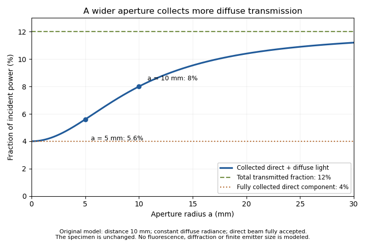
An unchanged hypothetical nail specimen gives different measured transmission as collection radius changes
. Original constant-radiance geometric model at distance 10 mm. The direct fraction is 4 percent and the diffuse fraction is 8 percent. These are stipulated values, not measured human-nail data. **Details**.

An aperture-scan separation of direct and diffuse nail transmission needs distinct acceptances and a stable angular model. In the ideal two-aperture case,

T_{s} = \frac{T ( a _{2} ) - T ( a _{1} )}{η _{2} - η _{1}}, T_{d} = T (a_{1}) - η_{1} T_{s} .

For the stated values, the two measurements recover 0.08 and 0.04. Nearly equal acceptances amplify measurement differences by a large factor. Changing distance or source size during the scan would change the model as well as the acceptance.

The primary nail experiment used an integrating sphere with a monochromator and photodiode to measure transmitted radiation.^[ref] The sphere provides a different angular collection arrangement from this opening model; it does not establish the assumed diffuse radiance law. A useful comparison characterizes each detector geometry before interpreting a signal difference as a change in the nail plate.

Aperture-scan separation of direct and diffuse nail transmission ( $Y_{j} = T_{d} + η_{j} T_{s}$ )

Aperture-scan separation of direct and diffuse nail transmission estimates the directly collected and diffusely transmitted fractions of light by changing detector acceptance while keeping the nail plate and illumination fixed. Separation depends on a stated angular model: a change in aperture is an experimental control, not a direct label attached to every photon.

In the original constant-diffuse-radiance model, let

Y_{j} = T_{d} + η_{j} T_{s} + ϵ_{j}

, where

T_{d}

is the fully accepted direct fraction,

T_{s}

the total diffuse fraction and

η_{j}

the known diffuse acceptance. For a coaxial circular opening, the geometric approximation gives

η_{j} = a_{j}^{2} / (a_{j}^{2} + r^{2})

. Two distinct acceptances give

T_{s} = \frac{Y _{2} - Y _{1}}{η _{2} - η _{1}}, T_{d} = \frac{η _{2} Y _{1} - η _{1} Y _{2}}{η _{2} - η _{1}} .

The distinction between these components is identifiable within this model only when the acceptances differ.

Suppose

η_{1} = 0.20

η_{2} = 0.50

Y_{1} = 0.056

and

Y_{2} = 0.080

. The fitted fractions are

T_{s} = 0.08

and

T_{d} = 0.04

. If independent signal errors each have standard uncertainty

σ = 0.002

, with acceptance uncertainty temporarily neglected, linear propagation gives

u^{2} (T_{s}) = \frac{2 σ ^{2}}{( η _{2} - η _{1} ) ^{2}}, u^{2} (T_{d}) = \frac{( η _{1}^{2} + η _{2}^{2} ) σ ^{2}}{( η _{2} - η _{1} ) ^{2}},

and

Cov (T_{d}, T_{s}) = - \frac{( η _{1} + η _{2} ) σ ^{2}}{( η _{2} - η _{1} ) ^{2}} .

The resulting uncertainties are about 0.00943 and 0.00359. Their negative covariance matters when adding the components: the total-transmission uncertainty is about 0.00629, rather than the value obtained by incorrectly treating the fitted components as independent.^[ref]

Additional apertures give a straight-line fit of

Y

against

η

, with intercept

T_{d}

and slope

T_{s}

. Weighted least squares can use independently characterized signal uncertainties. Systematic curvature would challenge the assumed angular law or fixed direct-beam acceptance. A plausible line alone does not prove that a finite source, changing geometry or residual fluorescence has been modeled correctly.

The primary nail-transmission study collected transmitted light using an integrating sphere, monochromator and photodiode.^[ref] The aperture scan here is an original proposed comparison, not a procedure or angular scattering law reported in that experiment.

Fluorescence contamination in nail-transmission measurements

Fluorescence contamination in nail-transmission measurements occurs when light emitted by a specimen contributes to a detector signal intended to quantify transmitted illumination. Emission can reach the detector at wavelengths different from the selected illumination wavelength, where detector spectral responsivity may also differ. Total current therefore need not be proportional to the desired transmitted power alone.

The primary human-nail experiment explicitly included a correction for nail fluorescence in its monochromator, integrating sphere and photodiode measurement.^[ref] It supplies an experimental motivation for distinguishing optical transmission from all detected light.

An original two-channel calibration model makes the separation explicit. Let

P_{t}

be transmitted excitation-band power and

P_{f}

an emitted component with a specified spectral shape. After dark-signal subtraction, calibrated channel readings satisfy

S_{1} = a_{1} P_{t} + b_{1} P_{f}, S_{2} = a_{2} P_{t} + b_{2} P_{f} .

The coefficients incorporate filters, detector spectral responsivity and collection efficiency. Separation requires

a_{1} b_{2} - a_{2} b_{1} \neq = 0

; two identical mixtures provide no additional information.

For stipulated dimensionless coefficients

(a_{1}, b_{1}) = (1, 1)

and

(a_{2}, b_{2}) = (0.1, 0.8)

, power-equivalent readings 0.100 and 0.024 mW give

P_{t} = \frac{0.8 ( 0.100 ) - 0.024}{0.7} = 0.080 mW, P_{f} = \frac{0.024 - 0.1 ( 0.100 )}{0.7} = 0.020 mW .

At incident power 1 mW, the corrected excitation-band transmittance is 8%; treating the first channel as transmission alone gives 10%. These are illustrative signals, not reported nail data.

Excitation-band selectivity in nail fluorescence corrections can be tested by changing the detection spectral band while keeping excitation and geometry fixed. The calibration still depends on the assumed emission spectrum: a different spectral shape can change the

b_{j}

coefficients. A filter can also reject some desired transmitted light, requiring its own calibration.

Separate dark current, stray excitation light and specimen emission in the measurement equation. A correction is useful only for the component it actually constrains; it should not be interpreted as identifying the chemical origin of all remaining optical changes.

Excitation-band selectivity in nail fluorescence corrections ( $i = a P_{t} + b P_{f}$ )

Excitation-band selectivity in nail fluorescence corrections describes how well the detection system distinguishes transmitted illumination from light emitted by the nail plate. Selecting the illumination with a monochromator does not force every detected photon to remain in that spectral band: fluorescence can contribute at other wavelengths.

For an original linear detection model, write the transmitted and emitted spectral powers as

P_{t} h (λ)

and

P_{f} f (λ)

, where both spectral shapes integrate to one. If an optical filter has transmission

τ (λ)

and a detector has spectral responsivity

R (λ)

, its current after subtraction of dark current is

i = \int R (λ) τ (λ) [P_{t} h (λ) + P_{f} f (λ)] d λ = a P_{t} + b P_{f} .

The coefficients

a, b

are spectrum-weighted responsivities, with units of amperes per watt. A selective filter can reduce

b

while also reducing

a

, so an uncorrected smaller current does not establish lower specimen transmittance.

For stipulated

a = 0.30 A/W

b = 0.020 A/W

P_{t} = 80 μ W

and

P_{f} = 20 μ W

, current is

24.4 μ A

. Assigning all of it to transmitted illumination gives

i / a = 81.33 μ W

, a 1.67% relative overestimate. These chosen coefficients illustrate leakage; they are not measured filter characteristics for nails.

Emission-spectrum mismatch in nail fluorescence subtraction matters when the assumed

f (λ)

differs from the specimen's emission. If analysis subtracts

b_{0} P_{f}

while the true coefficient is

b

, then

P_{t} - P_{t} = \frac{( b - b _{0} ) P _{f}}{a} .

At the same powers and

a

, using

b_{0} = 0.010 A/W

instead of 0.020 leaves a

0.667 μ W

positive bias. A precisely known total emitted power would not eliminate this spectral mismatch.

The historical nail-transmission experiment explicitly corrected for fluorescence.^[ref] The integral above is an explanatory extension, not a reconstruction of its unpublished correction coefficients. An experimental test would characterize detector/filter response and compare detection bands while keeping illumination and collection geometry in nail-transmission measurements fixed. Spectral rejection and angular collection constrain different parts of the measurement.

Emission-spectrum mismatch in nail fluorescence subtraction ( $Δ P_{t} = (b - b_{0}) P_{f} / a$ )

Emission-spectrum mismatch in nail fluorescence subtraction is the error caused by correcting a detector reading with an assumed fluorescence spectrum that differs from the actual emitted spectral shape. Knowing total fluorescent power does not generally determine fluorescent detector current, because the detector/filter response varies with wavelength.

Let

f (λ)

be the true normalized emission spectrum,

f_{0} (λ)

the assumed normalized spectrum and

k (λ) = R (λ) τ (λ)

the product of spectral responsivity and optical filter transmission. Define

b = \int k (λ) f (λ) d λ, b_{0} = \int k (λ) f_{0} (λ) d λ .

For a current

i = a P_{t} + b P_{f}

, subtraction of

b_{0} P_{f}

gives

P_{t} - P_{t} = \frac{P _{f}}{a} \int k (λ) [f (λ) - f_{0} (λ)] d λ .

Although

\int (f - f_{0}) d λ = 0

, the response-weighted integral need not vanish. Equal total emitted powers can therefore require different corrections.

An original two-band example makes the effect visible. Suppose the effective responsivity is

k_{1} = 0.30

and

k_{2} = 0.050 A/W

in two nonoverlapping bands. If fraction

q

of fluorescent power lies in the first band,

b (q) = k_{1} q + k_{2} (1 - q)

. The assumed fraction

q_{0} = 0.80

gives

b_{0} = 0.25 A/W

, whereas the true

q = 0.20

gives

b = 0.10 A/W

. At

P_{f} = 20 μ W

and transmitted-band responsivity

a = 0.30 A/W

, the transmitted-power estimate is biased by

- 10 μ W

. A true

80 μ W

would be reported as

70 μ W

after that excessive subtraction.

These are stipulated spectral shapes and coefficients, not measured nail spectra. If

k

were constant over the entire emission band, normalization would make this particular shape error vanish. A selective system generally sacrifices that invariance to distinguish transmitted excitation light from emission. Responsivity characterization and spectral measurement must therefore accompany a proposed subtraction.

The primary nail experiment explicitly included a correction for fluorescence while measuring transmission with a monochromator, integrating sphere and photodiode.^[ref] That observation motivates the distinction between emitted power and detected current; it does not specify the two-band correction model above. Fixing an assumed spectrum in software does not establish that the specimen actually has that spectrum.

Nail-plate material age from growth marks

Nail-plate material age from growth marks estimates how long a marked part of the nail plate has travelled since crossing a specified reference. It is a transport clock, not a direct observation of the instant when the material first formed in the nail matrix. The anatomical reference and any hidden travel before reaching it must be specified.

In a primary growth experiment, 22 young adults made file marks near the proximal fold, recorded their positions and repeated the measurements one to three months later.^[ref] This measures average displacement during the observation interval; it does not by itself recover every earlier growth rate.

For an original one-dimensional advection model, let a material element cross the reference at time

t_{0}

. If plate advance is spatially uniform with speed

v (t) > 0

, its later position is

x (t) = \int_{t_{0}}^{t} v (s) d s .

A known growth history permits inversion for

t_{0}

. A current speed alone need not. For example, 30 days at

0.08

mm/day followed by 30 days at

0.12

mm/day gives displacement 6 mm and age 60 days. Dividing by the final speed gives only 50 days, because it substitutes today's speed for the earlier history.

If only bounds

0 < v_{m i n} \leq v (s) \leq v_{m a x}

are justified throughout the travel, then

\frac{x}{v _{m a x}} \leq t - t_{0} \leq \frac{x}{v _{m i n}} .

For 6 mm and stipulated speeds between 0.08 and 0.12 mm/day, the reference-crossing age lies between 50 and 75 days. These bounds describe an original model, not published population limits.

A clipping also spans material positions. Even at a perfectly known constant speed of 0.10 mm/day, a 3 mm longitudinal segment spans 30 days of reference-crossing times. Temporal averaging in nail clippings therefore remains after instrument precision improves. External contamination or chemical exchange can further separate a measured chemical signal from the time of matrix production. Record mark position, reference fold, clipping extent and observation dates before treating a nail plate sample as a dated exposure record.

Temporal averaging in nail clippings

Temporal averaging in nail clippings is the mixing of material formed or transported at different times into one measured sample. A clipping has finite length, width and thickness. Even perfect chemical measurement of the whole sample need not resolve the timing of a short exposure.

A primary nail-growth experiment followed file marks near the proximal fold in 22 young adults over one to three months.^[ref] Such displacement measurements constrain the transport clock. Relating a chemical concentration to an earlier exposure requires additional assumptions about incorporation, retention and contamination.

For an original ideal advection model, let material cross a reference at time

s

with concentration

c (s)

, thereafter retained unchanged. At constant speed

v > 0

, a segment between positions

x_{1}

and

x_{2}

at collection time

t

contains reference-crossing times from

t - x_{2} / v

t - x_{1} / v

. If mass per unit length is uniform, its measured concentration is

\overline{c} (t) = \frac{1}{Δ} \int_{t - x_{2} / v}^{t - x_{1} / v} c (s) d s, Δ = \frac{x _{2} - x _{1}}{v} .

This is a shifted moving average, equivalently a convolution with a rectangular window. Its clock is reference crossing; formation in the hidden nail matrix may precede that crossing.

For a 3 mm segment at stipulated speed 0.10 mm/day,

Δ = 30

days. If a hypothetical incorporated concentration equals

C

for only five days and zero otherwise, the largest possible clipping average is

5 C /30 = C /6

. A broad, low measured peak can therefore result from a short, high input without any chemical decay. These values illustrate the model rather than an observed exposure record.

Spatial weighting of nail-clipping exposure records becomes important when thickness, width or density varies: the average is weighted by material mass, not distance alone. Variable growth further distorts the time window. A wider segment generally mixes a longer history, while repeated analyses of the same segment improve analytical precision without shortening that history.

Record clipping extent, material orientation, collection date and how growth was measured. Comparing several separately retained segments can provide more time information than pooling them, but recovering a unique exposure history remains an inverse problem unless the transport and retention model is sufficiently constrained.

Figure 1.
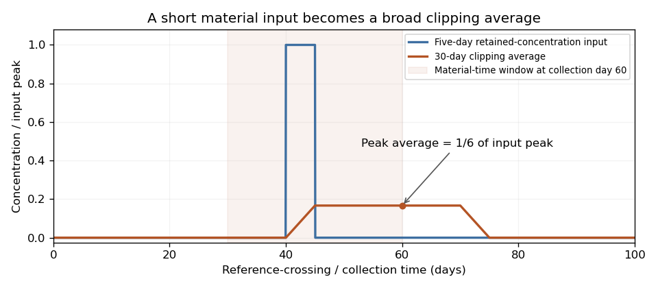
An original ideal clipping model spreads a five-day retained-concentration input across a thirty-day material window. The peak clipping average is one sixth of the input peak, even without chemical decay.
**Details**.

Spatial weighting of nail-clipping exposure records

Spatial weighting of nail-clipping exposure records determines how much each region of a clipping contributes to a pooled chemical measurement. A concentration reported per unit nail mass is a mass-weighted average. Equal lengths of nail plate need not supply equal amounts of material if width, thickness or density differs.

Let

m (x)

be mass per unit length at collection and

c (x)

the retained concentration per unit material mass. For a clipping spanning

[x_{1}, x_{2}]

, an original ideal recovery model gives

M = \int_{x_{1}}^{x_{2}} m (x) d x, \overline{c} = \frac{1}{M} \int_{x_{1}}^{x_{2}} m (x) c (x) d x .

This assumes complete, composition-independent recovery by the assay. If recovery varies spatially, the measurement equation requires that additional weighting.

For two equal-length regions with masses 1 and 3 mg and stipulated concentrations 0 and 100 units per mg, the pooled concentration is

(1 (0) + 3 (100)) / (1 + 3) = 75

units per mg. A length-weighted average would give 50 and answer a different question. The numerical example illustrates geometry and normalization, not an observed exposure.

Mass-normalized temporal kernels for nail clippings arise when positions are converted into earlier reference-crossing times. If

x = x (s)

is the material map at collection, the normalized time weighting is

w (s) = \frac{m ( x ( s )) ∣ d x / d s ∣}{M}, \overline{c} = \int w (s) c (s) d s .

At constant advance speed and uniform line density, the kernel is rectangular, recovering temporal averaging in nail clippings. Variable material geometry or speed changes its shape. A growth experiment following file marks measures displacement over a known interval, not this entire weighting function.^[ref]

A practical study retains segment orientation and measures the material amount used in each assay. Pooling several digits introduces further weights and potentially different growth histories. Wet-mass and structural-mass normalization also differ when water content changes, connecting the issue to hydration versus production in nail mass balance. Specify the denominator and material-to-time map before assigning a pooled concentration to one exposure date.

Mass-normalized temporal kernels for nail clippings ( $\int w (s) d s = 1$ )

Mass-normalized temporal kernels for nail clippings assign each earlier material time its fraction of the analyzed sample's mass. They convert a finite clipping into an averaging operator on a time-dependent retained concentration. The weighting is normalized by the assayed material amount, rather than by elapsed time alone.

For an original one-dimensional advection model, let

s

be the time when a material element crossed a defined anatomical reference, and collect at time

t

. With spatially uniform positive advance speed

v (u)

x (s) = \int_{s}^{t} v (u) d u, \frac{d x}{d s} = v (s) .

Suppose the clipping's retained elements correspond to

s \in [s_{1}, s_{2}]

. Let

m (x, t)

be structural mass per unit length at collection, and assume the marker's concentration per structural mass is preserved along each element. Then

M = \int_{s_{1}}^{s_{2}} m (x (s), t) v (s) d s, w (s) = \frac{m ( x ( s ) , t ) v ( s )}{M}, \overline{c} = \int_{s_{1}}^{s_{2}} w (s) c (s) d s .

The kernel has units of inverse time, is nonnegative and integrates to one. It can be treated mathematically like a probability density function for the reference-crossing time of material selected in proportion to its mass. This is a material-accounting interpretation, not a claim that the biological transport is random.

For a stipulated 20-day window, take line density 1 mg/mm, advance 0.10 mm/day in the earlier ten days and 0.20 mm/day in the recent ten days. The two intervals contribute 1 and 2 mg, respectively. Their kernel heights are

1/30

and

1/15

per day. A retained concentration of 90 ng/mg only in the earlier interval gives

\overline{c} = 30

ng/mg; a uniform time average would give 45. A constant 30 ng/mg history gives the same sample result. Thus one pooled measurement does not identify a unique history.

A centroid date of a mass-normalized nail kernel summarizes the weighting, while the kernel's spread records its finite time resolution. Neither removes the difference between reference crossing and earlier formation in the hidden nail matrix. The primary nail-marking experiment measures displacement over observation intervals, not the complete kernel or marker retention law.^[ref] Measuring segment mass, geometry and growth history constrains separate parts of this model.

Centroid date of a mass-normalized nail kernel ( $μ_{s} = \int s w (s) d s$ )

The centroid date of a mass-normalized nail kernel is the weighted mean of the reference-crossing times represented by the analyzed nail material. If

w (s) \geq 0

is normalized so that

\int w (s) d s = 1

, its centroid is

μ_{s} = \int s w (s) d s .

At collection time

t

, the corresponding mean material age is

\overline{a} = t - μ_{s}

. This summarizes a distribution of material times; it is not automatically the date of an exposure or the instant of formation in the nail matrix.

For an original pooled-sample example, suppose equal structural mass comes from two material-age intervals, 0–2 and 18–20 days before collection. Age density is 0.25 per day in each interval and zero between them. Their interval means are 1 and 19 days, so the mean age is 10 days. Yet no sampled material has age 10 days. A single uniform kernel over 0–20 days has the same mean age, with a very different distribution.

The age variance makes part of the difference explicit. A uniform interval of width 2 days has variance

2^{2} /12 = 1/3 da y^{2}

. The separated mixture therefore has

σ_{a}^{2} = \frac{1}{3} + \frac{( 1 - 10 ) ^{2} + ( 19 - 10 ) ^{2}}{2} = \frac{244}{3} da y^{2},

whereas a uniform 20-day interval has variance

2 0^{2} /12 = 100/3 da y^{2}

. Equal centroids do not imply equal temporal resolution.

Figure 1.
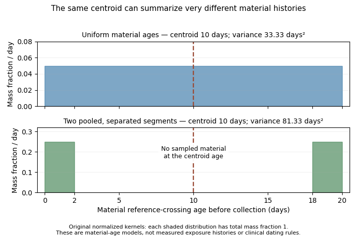
Two original material-age kernels have the same mean age but different spread and sampled intervals
. The lower kernel pools two separated segments of equal mass. Its mean age lies in a gap containing no sampled material. These are hypothetical reference-crossing ages, not observed exposure histories. **Details**.

The centroid has a precise averaging property. For any representative time

r

\int (s - r)^{2} w (s) d s = \int (s - μ_{s})^{2} w (s) d s + (r - μ_{s})^{2} .

It minimizes the mass-weighted squared timing discrepancy. Also, if retained concentration is affine in

s

, its kernel average equals its value at

μ_{s}

. This equality generally fails for a nonlinear history: a quadratic

c (s) = c_{0} + k (s - μ_{s})^{2}

averages to

c_{0} + k σ_{s}^{2}

, not

c_{0}

A primary growth experiment followed marks near the proximal nail fold over measured intervals.^[ref] Such displacement observations help constrain the material clock. They do not establish the full kernel, marker retention or one unique exposure date. Report the reference, distributional width and pooling assumptions alongside a centroid date.

Nail bed

The nail bed is the living supporting tissue beneath the attached nail plate. Its specialized epidermal region and underlying vascular support differ from the compact dead keratinized plate above it. The blood-rich tissue beneath the plate contributes the usual pink appearance.^[ref] The nail matrix near the root has the distinct growth-producing role.

This anatomy separates a material measurement from a view through that material. Light observed from a nail can depend on both the plate's optical properties and the tissue beneath it. The plate need not contain blood vessels for underlying vascular tissue to influence its appearance.

An original two-pass optical toy model writes the observed intensity as

I = I_{0} T^{2} R

, where

T

represents single-pass plate transmission and

R

the fraction returned by the underlying tissue. It ignores multiple scattering and detailed geometry. With stipulated

R = 0.5

, changing

T

from 0.8 to 0.6 changes

I / I_{0}

from 0.32 to 0.18 even though the underlying tissue parameter has not changed.

The calculation illustrates an inverse-problem limitation, not a clinical colour calibration. A change in appearance can reflect the covering plate, lighting, geometry or the underlying tissue. A single colour observation does not uniquely determine one vascular quantity. Optical contribution of the nail bed should therefore be interpreted with a measurement model specifying what is illuminated and detected.

A proposed anatomical observation compares transmitted or reflected appearance with a labeled view of the plate, root and supporting region under standardized lighting. Record whether the plate is attached and which region is observed. The location of a structure and the source of the optical signal are different pieces of evidence; neither should be inferred solely from the fact that the nail looks pink.

Optical contribution of the nail bed

The optical contribution of the nail bed is the portion of measured light associated with tissue beneath the nail plate, after accounting for illumination, the covering plate and collection geometry. The vascular tissue beneath the plate contributes to its ordinary pink appearance, while the compact plate itself consists of dead keratinocytes.^[ref] A colour measurement combines optical transport and anatomy rather than directly reporting a single blood quantity.

An original simplified reflectance model is

y = \frac{I}{I _{0}} = P + T^{2} R,

where

P

represents light returned by the plate and interfaces,

T

is single-pass plate transmittance and

R

is the fraction returned from the underlying region. The square represents outward and return passage through the plate. This deliberately omits detailed multiple scattering; it is an explanatory model, not a clinical calibration.

Even with known

P = 0

y = 0.32

can arise from

(T, R) = (0.8, 0.5)

(0.4, 0.8)

. One measurement cannot distinguish those pairs. For small changes with

P = 0

\frac{d y}{y} ≃ 2 \frac{d T}{T} + \frac{d R}{R} .

Thus a 1% relative change in plate transmittance contributes approximately a 2% relative signal change without any change in underlying reflectance. This is a concrete inverse problem.

A primary experiment separated one optical component physically: thirteen autopsy toenails were measured at fifteen wavelengths between 300 and 600 nm using a monochromator, integrating sphere and photodiode, with a correction for nail fluorescence.^[ref] Measuring an isolated plate constrains its transmission; it does not measure living nail-bed blood flow.

Plate-bed optical identifiability requires additional constraints: independent plate measurements, a specified spectral model or multiple collection geometries. More wavelengths help only if the added data constrain the unknowns; allowing an arbitrary new

T

and

R

at every wavelength preserves the ambiguity.

Plate-bed optical identifiability

Plate-bed optical identifiability asks whether the measured optical data uniquely separate the covering nail plate from the underlying nail bed within a specified model. Additional measurements help only if their dependence on the unknown quantities supplies independent information. This is an application of identifiability, beyond obtaining a good numerical fit.

For an original two-pass model without surface-return background,

y_{λ} = T_{λ}^{2} R_{λ}

, where

y

is normalized measured intensity,

T

plate transmittance and

R

effective underlying reflectance. With an independently unknown

T

and

R

at each wavelength,

n

spectral values give

n

equations for

2 n

unknowns. Choosing an admissible

T

determines a corresponding

R = y / T^{2}

; collecting a denser spectrum alone need not remove the ambiguity.

A deliberately restrictive example assumes known attenuation coefficients

μ_{1}, μ_{2}

, plate thickness

h

, and one wavelength-independent effective reflectance

r

. Taking

T_{j} = e^{- μ_{j} h}

gives

lo g y_{j} = lo g r - 2 μ_{j} h, h = \frac{l o g ( y _{2} / y _{1} )}{2 ( μ _{1} - μ _{2} )}, r = y_{1} e^{2 μ_{1} h} .

μ_{1} \neq = μ_{2}

, the ideal equations identify two parameters. At stipulated

μ_{1} = 1 m m^{- 1}

μ_{2} = 0.5 m m^{- 1}

h = 0.5

mm and

r = 0.8

, the signals are approximately 0.2943 and 0.4852 and inversion recovers the chosen parameters. This exponential example is not a validated transport law for a living nail.

Spectral-contrast conditioning in nail optics distinguishes mathematical uniqueness from usable precision. With independent errors in the logarithmic signals,

Var (h) ≃ \frac{Var ( l o g y _{1} ) + Var ( l o g y _{2} )}{4 ( μ _{1} - μ _{2} ) ^{2}} .

Nearly equal coefficients amplify noise. At equal coefficients, the ideal inversion fails altogether. An unknown spectral shape of

R_{λ}

, surface return or additional multiple scattering introduces further unknowns.

A primary transmission study measured isolated autopsy nails using a monochromator, integrating sphere and photodiode, including a fluorescence correction.^[ref] Isolated-plate measurements illustrate how an independent experiment can constrain one component. They do not by themselves identify living nail-bed blood flow. State which quantities are independently measured and which are assumed before interpreting a fitted tissue parameter.

Spectral-contrast conditioning in nail optics

Spectral-contrast conditioning in nail optics describes how measurement errors are amplified when thickness or tissue parameters are recovered from spectral differences. A model can be identifiable in exact arithmetic while its parameter estimates are too sensitive to small signal or calibration errors to be useful.

For the original simplified plate model

y_{j} = r e^{- 2 μ_{j} h}

with known coefficients and wavelength-independent effective reflectance

r

, thickness is

h = \frac{l o g ( y _{2} / y _{1} )}{2Δ μ}, Δ μ = μ_{1} - μ_{2} .

Let each log signal have standard uncertainty

σ

and their correlation be

ρ_{e}

. The first-order thickness uncertainty is

u (h) ≃ \frac{σ 2 ( 1 - ρ _{e} )}{2 ∣ Δ μ ∣} .

The covariance term belongs to the uncertainty calculation; treating every spectral error as independent can be misleading.^[ref]

With stipulated

σ = 0.01

and independent errors, coefficient differences

0.5

and

0.05 m m^{- 1}

give thickness uncertainties about 0.0141 and 0.141 mm, respectively. A tenfold loss of spectral contrast produces tenfold error amplification. At the larger contrast and correlation 0.9, the modeled uncertainty is approximately 0.00447 mm. These are local model calculations, not validated precision claims for nail measurements.

Coefficient calibration also matters. If signal-ratio error and

Δ μ

error are independent,

u^{2} (h) ≃ \frac{u ^{2} ( l o g ( y _{2} / y _{1} ))}{4 ( Δ μ ) ^{2}} + h^{2} \frac{u ^{2} ( Δ μ )}{( Δ μ ) ^{2}} .

Collecting more signal averages does not eliminate the second term when the same uncertain calibration is reused.

Offset sensitivity of log-ratio nail models distinguishes error types. A common multiplicative factor cancels from

g y_{2} / (g y_{1})

; a common additive offset generally does not cancel from

(y_{2} + b) / (y_{1} + b)

. Background light or unseparated fluorescence can therefore bias an otherwise precise ratio. The primary nail-transmission experiment explicitly included a fluorescence correction.^[ref]

Choose spectral channels using both sensitivity and a defensible optical model. A strong contrast is not sufficient if the assumed plate coefficients, collection geometry or underlying spectral behaviour are wrong.

Offset sensitivity of log-ratio nail models ( $\partial h / \partial β$ )

Offset sensitivity of log-ratio nail models describes the bias produced when an additive background enters a ratio used to estimate a nail plate parameter. A shared multiplicative gain cancels from an ideal ratio, whereas a shared additive term generally remains.

Consider the original simplified spectral model

y_{j} = r e^{- 2 μ_{j} h}

, with plate thickness

h

, known attenuation coefficients

μ_{j}

and wavelength-independent effective reflectance

r

. Write

Δ μ = μ_{1} - μ_{2} \neq = 0

. The ideal thickness is

h = lo g (y_{2} / y_{1}) / (2Δ μ)

. If measured signals are

s_{j} = g y_{j} + b

with

g > 0

, define the input-equivalent offset

β = b / g

. Ignoring that offset gives

h = \frac{l o g [( y _{2} + β ) / ( y _{1} + β )]}{2Δ μ}, h - h = \frac{l o g ( 1 + β / y _{2} ) - l o g ( 1 + β / y _{1} )}{2Δ μ} .

Both offset-adjusted signals must be positive. Equal additive errors do not cancel inside this logarithm.

With stipulated

r = 0.8

h = 0.5

mm,

μ_{1} = 1 m m^{- 1}

and

μ_{2} = 0.5 m m^{- 1}

, the signals are about 0.2943 and 0.4852. Adding

β = 0.020

gives an apparent thickness of about 0.4746 mm. Positive background pulls the ratio towards one and underestimates thickness in this example. The numbers are model calculations, not an experimentally validated nail-thickness calibration.

The local sensitivity is

\frac{\partial h}{\partial β} = \frac{1}{2Δ μ} (\frac{1}{y _{2} + β} - \frac{1}{y _{1} + β}) .

At zero offset in the example it is approximately

- 1.337 mm

per unit normalized signal. A residual-offset standard uncertainty of 0.005 therefore contributes approximately 0.00668 mm to the local thickness uncertainty. If that same uncertain background correction is reused across channels, its errors are correlated; the covariance terms belong in the propagation model.^[ref]

Residual-offset uncertainty in nail thickness estimates remains even when repeated photon measurements reduce random fluctuations. A useful test measures dark current and examines optical background separately, since fluorescence need not have the same spectral dependence as either. The primary nail-transmission study explicitly included a fluorescence correction.^[ref] That motivates identifying the background component; it does not validate this reduced thickness model.

Residual-offset uncertainty in nail thickness estimates ( $u (h)$ )

Residual-offset uncertainty in nail thickness estimates is the uncertainty contributed by an imperfectly known additive background after correction of spectral signals. It differs from a known uncorrected offset's bias: subtraction can remove the best estimate of a background while leaving uncertainty about that estimate.

For an original reduced optical model, let two measured normalized signals be

Y_{1}, Y_{2}

and subtract the same background estimate

B

. Define

Z_{j} = Y_{j} - B > 0

and suppose the attenuation contrast

D = μ_{1} - μ_{2} \neq = 0

is known. The inferred nail plate thickness is

h = \frac{l o g ( Z _{2} / Z _{1} )}{2 D} .

Its sensitivity coefficients are

\frac{\partial h}{\partial Y _{1}} = - \frac{1}{2 D Z _{1}}, \frac{\partial h}{\partial Y _{2}} = \frac{1}{2 D Z _{2}}, \frac{\partial h}{\partial B} = \frac{1}{2 D} (\frac{1}{Z _{1}} - \frac{1}{Z _{2}}) .

With mutually independent raw signal estimates and background estimate, first-order uncertainty propagation gives

u^{2} (h) = \frac{1}{4 D ^{2}} [\frac{u ^{2} ( Y _{1} )}{Z _{1}^{2}} + \frac{u ^{2} ( Y _{2} )}{Z _{2}^{2}} + (\frac{1}{Z _{1}} - \frac{1}{Z _{2}})^{2} u^{2} (B)] .

This follows the sensitivity-and-covariance approach in the measurement guide.^[ref]

For stipulated

Z_{1} = 0.30

Z_{2} = 0.50

D = 0.50 m m^{- 1}

u (Y_{1}) = u (Y_{2}) = 0.003

and

u (B) = 0.010

, the estimated thickness is approximately 0.5108 mm and its combined standard uncertainty is 0.0177 mm. The common-background contribution alone is 0.0133 mm. Averaging 100 independent repetitions of each raw signal while reusing the same background estimate reduces the total only to about 0.0134 mm; it does not reduce that shared contribution by ten.

An equivalent calculation treats corrected signals as correlated:

Cov (Z_{1}, Z_{2}) = u^{2} (B)

under the stated independence assumptions. Omitting this covariance would describe a different experiment with independent background errors. Near zero corrected signal, the logarithm also becomes strongly nonlinear, so this local approximation needs further checking.

The primary nail experiment included a fluorescence correction in its optical transmission measurement.^[ref] Background emission and dark current must be characterized separately when they have different spectral responses. The equations above are an illustrative uncertainty budget, not a validated thickness calibration or reported precision from that experiment.

Nail matrix

The nail matrix is the proliferative growth region near the nail root that produces material incorporated into the nail plate. Cells divide and become keratinized as the resulting plate advances towards the fingertip. It is distinct from the supporting nail bed and from the free edge already exposed beyond the fingertip.^[ref]

An original steady-volume model links production to motion. Let

J

be net plate-material volume supplied per day,

w

the plate width,

h

its thickness and

v

its advance speed. If material is approximately incompressible, the cross-section is uniform and losses before the free edge are negligible,

J = w h v, v = \frac{J}{w h} .

For stipulated

J = 0.30 m m^{3} /day

w = 10

mm and

h = 0.30

mm, the advance is 0.10 mm/day. Doubling width at the same production and thickness halves that modeled advance. These are geometric consequences of a chosen model, not universal differences between individuals.

Matrix growth and plate-advection balance also shows why a measured advance speed does not alone determine a cell-division rate. Cell size, keratinization, plate geometry and the spatial distribution of production enter the conversion from proliferation to material flow. A marker on the plate measures movement of produced material.

A primary study measured nail advance using marks in 22 healthy young adults; the reported mean fingernail rate was 3.47 mm/month and mean toenail rate 1.62 mm/month.^[ref] Those measurements establish cohort growth observations, not direct counts of mitoses in the matrix.

A proposed comparison combines marked-plate displacement with measurements of plate width and thickness, keeping the observation interval and reference fold fixed. Interpreting changes in the inferred production rate requires checking the steady-geometry assumptions. The central anatomical distinction remains: the matrix supplies new material, while the mature plate records the movement and subsequent history of that material.

Matrix growth and plate-advection balance

Matrix growth and plate-advection balance relates newly supplied nail material to movement and changing geometry of the nail plate. The nail matrix contains the growth-producing region, whereas the mature nail plate is transported material.^[ref] Measured advance is consequently a material-flow observation, not a direct count of cell divisions.

For an original one-dimensional conservation of mass model, define line density

m (x, t) = ρ (x, t) A (x, t)

, where

A

is plate cross-sectional area,

ρ

its density and

v

its advance speed. A local production rate

s (x, t)

per unit length gives the continuity equation

\frac{\partial m}{\partial t} + \frac{\partial ( m v )}{\partial x} = s .

If the chosen downstream segment has negligible production or loss,

s = 0

. At steady state its mass flux

m v

is constant. Uniform density then makes the volume flux

Q = A v

constant, recovering the simple width-times-thickness model.

For stipulated

Q = 0.30 m m^{3} /day

, cross-sectional areas of 3 and

2 m m^{2}

require speeds 0.10 and 0.15 mm/day. Equal production can therefore accompany unequal advance when geometry changes. Conversely, equal speeds do not establish equal production without knowing area and density.

For a fixed segment

[a, b]

, integrating the continuity equation gives

\frac{d}{d t} \int_{a}^{b} m d x = (m v) (a, t) - (m v) (b, t) + \int_{a}^{b} s d x .

If inflow exceeds outflow, material accumulates rather than vanishing from the accounting. Growth, hydration-related geometry change and clipping must be assigned to appropriate terms before interpreting an apparent imbalance.

The nail-marking study measured displacement over known time intervals in 22 young adults.^[ref] Extending that design with repeated width and thickness measurements would test a nail-plate storage balance, rather than assuming steady geometry. Inferring a mitotic rate would require further information about cell size and conversion into mature material.

Nail-plate storage balance

Nail-plate storage balance accounts for material accumulating in a chosen nail plate segment when production and removal are unequal. A measured advance speed is a boundary-transport observation; it does not alone specify how much material is stored or produced.

For an original fixed-segment mass conservation model, let

M (t)

be stored structural mass,

F_{in}

and

F_{out}

its boundary fluxes,

P

local production and

L

other losses. Then

\frac{d M}{d t} = F_{in} - F_{out} + P - L .

This is the integrated continuity equation. If production is confined outside the selected segment,

P = 0

there even though the upstream nail matrix continues producing material. Moving the measurement boundary changes which processes appear as local production or inflow.

With constant density, an illustrative volume version has inflow

0.30 m m^{3} /day

and outflow

0.24 m m^{3} /day

, giving storage gain

0.06 m m^{3} /day

. After ten days the gain is

0.60 m m^{3}

. Spread over a fixed

10 \times 20 m m^{2}

footprint, that corresponds to an average thickness increase of 0.003 mm. These are geometric consequences of the chosen model, not measured nail-growth constants.

Clipping is a discrete loss. If a clipping of mass

m_{c}

is removed at time

t_{c}

, the balance includes

M (t_{c}^{+}) = M (t_{c}^{-}) - m_{c}

. A smooth growth curve fitted across this jump could misinterpret removal as decreased production. Repeated position measurements should therefore be accompanied by clipping records.

Hydration versus production in nail mass balance separates structural material from water:

M_{wet} = M_{structural} + M_{water}

. A rise in wet mass need not mean new structural material. A primary ellipsometry experiment measured changes in the complex refractive index of human fingernails during water uptake and loss, using a model with more weakly and more tightly associated water.^[ref] That establishes a conditioning-dependent material response, not matrix proliferation.

A useful experiment measures marked displacement, segment geometry and mass under matched conditioning while recording removals. The measurement model must identify whether it tracks wet material, structural material or an optical proxy; these are different storage quantities.

Hydration versus production in nail mass balance

Hydration versus production in nail mass balance distinguishes changes in retained water from changes in structural nail plate material. A wet mass, a thickness reading and a marked displacement measure different properties. They cannot be converted into a common production rate without a model of composition and geometry.

Write an original two-inventory balance as

M_{wet} = M_{s} + W, \frac{d M _{s}}{d t} = P_{s} - L_{s}, \frac{d W}{d t} = J_{w, in} - J_{w, out} .

Here

M_{s}

is structural mass,

W

retained water, and

P_{s}, L_{s}

structural production and loss. Wet-mass gain can occur with

P_{s} = 0

when water inflow exceeds outflow. For an isolated clipping, there is no continuing supply from the nail matrix even though water exchange can continue.

A primary ellipsometry study measured changes in human fingernail complex refractive index during water uptake and loss, reporting characteristic time domains of approximately 4, 150 and 3,200 minutes. Its model distinguished more weakly and more tightly associated water in keratin.^[ref] Those observations concern material conditioning; they are not measurements of matrix cell production or universal time constants for every nail.

For a simple illustrative one-pool relaxation,

W (t) = W_{\infty} + (W_{0} - W_{\infty}) e^{- t / τ}

. Choose fixed

M_{s} = 10

mg,

W_{0} = 4

mg,

W_{\infty} = 2

mg and

τ = 60

minutes. Wet mass falls from 14 towards 12 mg, reaching approximately 12.736 mg after one hour, despite unchanged structural material. These values are constructed examples rather than fitted parameters from the cited study.

Water-denominator effects in nail concentration measurements follow even if a retained marker amount is unchanged. A stipulated 100 ng marker in those samples would increase from

100/14 \approx 7.14

100/12 \approx 8.33 ng m g^{- 1}

when expressed per wet mass, a 16.7% increase without added marker. Actual retention must be checked rather than assumed.

A useful experiment records conditioning, weighs the sample over time and independently measures geometry or optical response. Structural production, water exchange and clipping removal belong to separate terms. Specify whether a reported concentration is normalized to wet material or a separately characterized structural amount before comparing measurements.

Water-denominator effects in nail concentration measurements ( $C_{wet} = A / (M_{s} + W)$ )

Water-denominator effects in nail concentration measurements occur when a concentration changes because the amount of retained water changes the sample mass used for normalization. This can happen without any change in the amount of the measured substance. The denominator is part of the reported observable.

For an original inventory model, let

A

be the retained marker amount,

M_{s}

structural mass and

W

water mass. Define the water fraction of wet material as

f = W / (M_{s} + W)

. Concentrations on the two stated bases obey

C_{wet} = \frac{A}{M _{s} + W}, C_{s} = \frac{A}{M _{s}}, C_{wet} = (1 - f) C_{s} .

At fixed

A

and

M_{s}

, increasing hydration lowers

C_{wet}

while leaving

C_{s}

unchanged. The structural basis here is a model-defined material amount; an actual drying procedure must establish what it retains before being equated with

M_{s}

For stipulated

A = 100

ng and

M_{s} = 10

mg, increasing

W

from 2 to 5 mg changes the wet-basis concentration from

100/12 = 8.33

100/15 = 6.67

ng/mg, a 20% decrease. Both concentrations correspond to 10 ng/mg on the structural basis. Comparing the wet values alone would falsely suggest a marker loss if unchanged hydration were assumed.

The relation also affects pooled samples. Take two clippings with equal structural mass 10 mg and equal marker amount 100 ng, but water amounts 0 and 10 mg. Their wet-basis concentrations are 10 and 5 ng/mg. Pooling gives

200/30 = 6.67

ng/mg, rather than the unweighted average 7.5. Mass-normalized temporal kernels for nail clippings must therefore use the same mass basis as the constituent concentrations.

A further assay factor can change the numerator as well. If a fraction

q

of the retained marker is recovered, the measured quantity is

q A / (M_{s} + W)

. Correcting water content cannot by itself establish

q = 1

or prove that

A

stayed constant. An original comparison should independently track conditioning, sample mass and recovery before attributing a concentration difference to changed incorporation.

A primary ellipsometry experiment observed the complex refractive index of fingernails during hydration and dehydration, relating the response to water associated with keratin.^[ref] This supports treating hydration as a material-state variable. The denominator equations follow from conservation of mass; the optical experiment does not directly measure marker retention or matrix production.

Thymus

The thymus is an organ of the lymphatic system involved in development of T cells. In humans it lies in the chest behind the sternum. Its anatomical position and its contribution to immunity are different properties: locating an organ does not by itself reveal its function.^[ref]

A motivating experiment removed the thymus from newborn mice. In his firsthand account, Jacques Miller describes finding a deficiency of lymphocytes in other lymphoid tissues and failure to reject foreign skin grafts. Supplying circulating lymphocytes or a thymus graft could restore the graft-rejection response. Removal, a functional test and rescue together connected the thymus with development of immune competence.^[ref]

A further comparison separated two consequences. In germ-free conditions, mice subjected to neonatal thymectomy could remain healthy yet still fail to reject skin grafts. Thus wasting illness and the measured graft-rejection defect were not interchangeable observations.^[ref]

For an original experimental-design outline, compare sham-operated and thymectomized animals under matched conditions, then score lymphocyte abundance, health and graft rejection separately. Include a defined rescue condition. These endpoints distinguish loss of immune competence from a nonspecific effect of surgery. The neonatal timing matters: an experiment on development does not justify assuming that removal at every age has identical effects.

Thymectomy

Thymectomy is surgical removal of the thymus; the term must be qualified when removal is partial rather than complete. In an experiment it is an intervention on an organ, whose effect is assessed through separately defined anatomical and functional outcomes.

Its scientific importance is illustrated by neonatal experiments described firsthand by Jacques Miller. Mice whose thymus had been removed at birth showed deficient lymphocyte populations and failed to reject foreign skin grafts. Supplying a thymus graft or circulating lymphocytes restored immune responsiveness in the reported comparisons.^[ref]

Completeness and timing changed interpretation. Miller recounts that partial removal helped explain why some investigators did not reproduce the full graft-acceptance phenotype. He also distinguishes neonatal removal from removal in adults. The name of an intervention alone therefore does not specify either its anatomical extent or the developmental state in which it was performed.^[ref]

For an original controlled comparison, keep sham-operated, partially thymectomized and completely thymectomized groups distinct, then measure lymphocyte abundance and skin graft rejection separately. A rescue group tests whether restoring a missing contribution also restores the response. These observations support a causal role more directly than a correlation between organ size and illness. They do not establish that surgery has identical effects at every age or in every species.

Tetrapod limb

A tetrapod limb is a paired appendage of a tetrapod, such as a forelimb or hindlimb, organized around a shared inherited skeletal pattern. In a familiar forelimb, one proximal bone, the humerus, is followed by the radius bone and ulna, then more distal elements and limb digits. The corresponding structures can differ greatly in proportions and use. Comparing their relationships, rather than just their overall shape, is central to recognizing homology.

The transition from a fin to a limb was not an instantaneous appearance of an entire new skeleton. A 2006 study of Tiktaalik described a pectoral fin with an expanded distal internal skeleton and articulations permitting a substrate-supported posture. The reconstructed joint configurations included flexed shoulder and elbow regions and an extended distal region. This indicates precursors of limb-like support in a finned animal; it does not make every distal fin element a limb digit.^[ref]

A useful comparison traces the humerus, radius bone and ulna in two differently shaped forelimbs, then asks which elements contact one another. A wing and a walking appendage can preserve corresponding elements while redistributing their lengths and mechanical roles. Shared ancestry and present function are related questions, but one cannot be read directly from the other.

Limb digit

A limb digit is one of the terminal rays of a tetrapod limb, such as a finger or toe. A digit includes a series of phalanges and surrounding tissues; it is not synonymous with one phalanx. Several bones can therefore belong to one digit, with a joint connecting successive elements.

Counting digits and counting their component bones answer different questions. If a hypothetical limb has five digits and each has three phalanges, it has five digital rays but fifteen phalangeal bones. This deliberately simplified example shows why an isolated row of bones must first be reconstructed into its anatomical arrangement before it is used to infer digit number.

Nor is five digits the defining ancestral condition of every early tetrapod limb. In 1990, fossil descriptions documented eight digits in the forelimb of Acanthostega, while other early specimens had different counts. These observations challenged reconstructions that began by assuming an originally fixed five-element pattern. The specimens are evidence about the early diversity of limbs, rather than abnormal individuals judged against the human hand.^[ref]

Lumen (anatomy)

A lumen is the internal space of a hollow organ or vessel. In a blood vessel, the lumen contains the flowing blood and is bounded by endothelium. In the small intestine, the lumen contains material being digested and is bounded by an epithelium. The space, its contents and its surrounding wall are distinct anatomical objects.^[ref]

A transverse section makes the distinction visible. Model a circular tube with inner radius

r

and outer radius

R

, where

R > r

. The luminal cross-sectional area is

π r^{2}

, whereas the wall occupies

π (R^{2} - r^{2})

. If

R = 2 r

, the wall's cross-sectional area is three times the luminal area. Measuring the outside of a tube therefore does not directly measure its internal opening.

For a lining epithelium, the apical membrane faces the lumen; its opposite side faces underlying tissue. This orientation explains why transport into the lumen and transport into the surrounding interstitial fluid are physiologically different directions, even when the same substance moves across the same layer of biological cells.^[ref]

Tubular lumen

A tubular lumen is the continuous internal passage of a tube-shaped anatomical structure. In a renal tubule, its lining epithelium separates the tubular fluid from surrounding interstitial fluid. The apical membrane faces the tubular lumen, so movement along the tube and movement across its wall follow different paths.^[ref]

A straight cylinder gives a useful scale estimate. If the internal radius is

10 μ m

and the length is

1 mm

, the luminal volume is

V = π r^{2} L = π (10 μ m)^{2} (1000 μ m) \approx 0.314 nL .

This is an ideal geometric example; real renal tubules change shape and diameter along their length.

Experiments on isolated perfused collecting ducts exploit the same compartment distinction. Fluid is supplied through the tubular lumen, while a separate surrounding solution contacts the outside of the epithelium. Changing the conditions permits measurement of water crossing the wall. In a 1995 study, the increased membrane permeability during vasopressin exposure accompanied movement of aquaporin-2 toward the apical membrane.^[ref]

Mouth

The mouth is the entrance to the digestive tract and a movable part of the vocal tract. Its cavity is bounded by the lips, cheeks, palate and floor of the mouth, with the tongue occupying much of the space. The teeth break food into smaller pieces while the tongue and cheeks position it for chewing and swallowing.^[ref]

Mechanical processing and chemical processing cooperate: mixing food with saliva makes a movable bolus and exposes it to salivary components. The same cavity also changes shape during speech. Opening the jaw or repositioning the tongue changes the passage through which air and sound travel, so digestive anatomy is also an articulatory instrument.

Lip

A lip is a movable fold at the entrance to the mouth, with skin externally and oral mucosa internally. The lips contain the orbicularis oris muscle, whose contraction helps close and shape the oral opening. Their sensory supply helps guide contact with food and objects.^[ref]

The oral seal has several functions. During eating it helps retain food; during speech, closure and release can interrupt airflow, while rounding changes the geometry of the vocal tract. A bilabial stop such as /p/ uses contact between both lips, whereas a rounded vowel uses an open but reshaped outlet. The visible fold and the muscle controlling it are related structures, rather than identical anatomical objects.

Orbicularis oris muscle

The orbicularis oris muscle is a complex of skeletal muscle fibres around the mouth that closes and shapes the lips. Its contraction can press the lips together or project them forward. Compare sealing the mouth while holding water with rounding the lips to whistle: both use the same muscular region to change the outlet's shape. The visible lip includes other tissues besides the muscle that moves it.^[ref]

Anatomical lumen

An anatomical lumen is the internal space of a hollow organ or tubular structure. Blood occupies the lumen of a blood vessel, while intestinal contents occupy the lumen of the gut. The word identifies a space, not its wall, contents or diameter.

For a tube lined by epithelium, the apical cell surface faces the lumen and the basolateral surface faces the underlying tissue. This orientation matters for membrane transport: a substance can cross one side of a cell and leave through the other. In a nephron, for example, moving a solute from tubular lumen back toward the blood is reabsorption.

The gut illustrates why geometrical location and physiological access differ. Material can be inside the outline of the body yet still be in a lumen separated from internal tissues by an epithelial barrier. Absorption requires crossing that barrier. This anatomical meaning is separate from the photometric unit called the lumen.

Vocal tract ( $f_{n} ≃ (2 n - 1) c / (4 L)$ )

The vocal tract is the air passage above the sound-producing region of the larynx, including the pharyngeal, oral and, when acoustically coupled, nasal cavities. Movements of the tongue, lips, jaw and soft palate change its shape. These changes help turn a laryngeal sound source or a turbulent air stream into distinguishable speech sounds.^[ref]

A simple acoustic model treats an unbranched tract of length

L

as a uniform tube closed at one end and open at the other. A pressure maximum at the closed end and pressure minimum at the open end allow odd quarter wavelengths, giving

f_{n} = \frac{( 2 n - 1 ) c}{4 L}, n = 1, 2, \dots .

With

L = 0.17

m and sound speed

c = 340

m/s, these resonances are

500

1500

and

2500

Hz. A real vocal tract is neither uniform nor permanently closed at the glottis; its varying cross-section and branching shift the resonances. These spectral resonances, associated with formants, differ from the repetition frequency of vocal-fold vibration. This is why changing articulation can change a vowel without requiring the same change in voice pitch.

Prostate

The prostate is a gland below the male urinary bladder, surrounding the proximal urethra. Its secretions contribute to semen. This relationship to the urinary passage explains why a change in prostatic size can affect urine flow even though its secretory role is reproductive.

Anatomical trunk

The anatomical trunk is the main body region excluding the head, neck and limbs. In a human, it contains the thorax, abdomen and pelvis, with supporting structures and many major organs. The regional term organizes location rather than denoting one organ system.

Hilum

The region of an organ where principal vessels, ducts or other connections enter or leave; its contents depend on the organ.

Human skeleton

The human skeleton is the framework of bones that supports the body, protects organs and supplies attachment points for muscles. The axial skeleton includes the skull, vertebral column and rib cage; the appendicular skeleton includes the limbs and their girdles. Movement depends on this framework interacting with joints and tendons.

Exoskeleton

An exoskeleton is an external supporting or protective structure of an organism. An arthropod's chitinous exoskeleton supports muscle forces while also forming an outer barrier. Growth can therefore require a moult, linking the mechanical advantages of a rigid covering to a developmental constraint.

Chitinous exoskeleton

A chitinous exoskeleton is an external covering whose structural material includes chitin, commonly embedded in a protein matrix. In arthropods, regional differences in thickness and stiffness allow strong plates to coexist with flexible joints. Chitin is one component rather than a claim that the covering is chemically pure.

Penis

 1  0

The penis is an external organ containing the terminal urethra and erectile tissue. In human anatomy it participates in urinary outflow and reproductive delivery. Its vascular erectile mechanism is distinct from the neural and muscular coordination of ejaculation.

Perineum

The perineum is the region below the pelvic diaphragm between the thighs. Its anterior urogenital triangle and posterior anal region contain structures involved in urinary, reproductive and bowel functions. The region should be distinguished from the deeper pelvic cavity and from the perineal body within it.

Pelvic diaphragm

The pelvic diaphragm is the muscular floor of the pelvis, formed chiefly by the levator ani group and coccygeus with their associated fascia. It supports pelvic organs while allowing passages for the bowel and urogenital structures. Support and controlled passage must therefore be accommodated by one anatomical arrangement.

Pudendal canal

The pudendal canal is a passage in the fascia of obturator internus along the lateral perineal region. It carries the pudendal nerve and internal pudendal vessels. Their common route explains how a local anatomical lesion can affect both neural supply and vascular structures.

Perineal body

The perineal body is a fibromuscular junction in the perineum where several muscle and connective-tissue elements meet. In female anatomy it lies between the vagina and anal canal. Its value as a support point follows from the convergence of attachments, rather than from being a separate large muscle.

Urogenital triangle

The urogenital triangle is the anterior subdivision of the perineum. It contains the external urogenital openings and associated muscles and membranes. Its name identifies a topographic region; it is not synonymous with the older, anatomically misleading concept of a uniform urogenital diaphragm.

Urogenital diaphragm

Historical anatomical model of perineal muscle and fascia; it should not be read as a universally uniform muscular sheet between two identical fascial layers.

Perineal membrane

The dense fibrous membrane separating superficial and deeper perineal structures; corresponds to the inferior layer of older triangular-ligament descriptions.

Aortic hiatus

The aortic hiatus is the passage behind the respiratory diaphragm through which the aorta continues into the abdomen. Its location differs from the more anterior oesophageal hiatus. Separating the openings helps explain how major structures cross the thoracic-abdominal boundary along different routes.

Mediastinum

The mediastinum is the central compartment of the thorax between the pleural sacs. It contains the heart, major vessels, trachea, oesophagus and other structures. The lungs occupy the adjacent pleural regions, so an abnormality described as mediastinal is not automatically within lung tissue.

Obturator canal

The obturator canal is a short passage at the upper margin of the obturator opening in the pelvis. It transmits the obturator nerve and associated vessels toward the medial thigh. Its restricted route links pelvic anatomy to the nerve supply of thigh adductor muscles.

Radial groove

The radial groove is a groove on the posterior humerus associated with the course of the radial nerve and profunda brachii vessels. Their close relation to the bone helps explain why an injury of the humeral shaft can also disturb nerve function.

Gingiva

The gingiva is the gum tissue surrounding the teeth and covering the supporting alveolar region. It contributes a protective interface around each tooth. Its attached portions differ mechanically from the more mobile buccal mucosa.

Buccal mucosa

The buccal mucosa is the mucous membrane lining the inside of the cheek. It provides a flexible epithelial surface exposed to friction during mastication. It should be distinguished from the cheek's underlying buccinator muscle and from the gingiva around the teeth.

Infratemporal fossa

The infratemporal fossa is a deep space below the temporal region and medial to the mandibular ramus. It contains muscles, vessels and nerves associated with mastication, including parts of the pterygoid musculature. Its importance lies in the relations among these crowded structures rather than a visible external boundary.

Petrotympanic fissure

The petrotympanic fissure is a narrow opening in the temporal bone connecting the middle-ear region with the infratemporal region. The chorda tympani passes through it. This supplies a route by which a nerve associated with the facial nerve reaches structures outside the ear.

Stylomastoid foramen

The stylomastoid foramen is an opening in the temporal bone between the styloid and mastoid processes. The facial nerve exits the skull through it. Damage near the opening can therefore affect facial motor output after the nerve's earlier intratemporal course.

Ear

The ear is the sensory apparatus associated with hearing and, in its inner-ear components, balance. The outer and middle ear transmit sound mechanically toward the inner ear, where specialized sensory biological cells transduce movement into neural signals. Sound transmission and vestibular sensing are related anatomically but are different functions.

Inner ear

 1  0

The inner ear contains fluid-filled sensory structures for hearing and balance. In the cochlea, motion transmitted from the middle ear creates a traveling disturbance along the basilar membrane. Movement of sensory hair cells bends their stereocilia, changing mechanically gated ion-channel opening and producing an electrical response.^[ref]

The mechanical response varies along the cochlea, so position contributes to frequency selectivity. The vestibular part of the inner ear instead detects head motion and orientation. The distinction is anatomical and functional: detecting a sound frequency and detecting a rotation of the head use related mechanosensory principles in different structures. Mechanical input, hair-cell response and activity in the associated sensory neurons are successive measurable stages.

Tympanic membrane

The tympanic membrane is the thin membrane separating the external ear canal from the middle ear. Sound-pressure differences make it vibrate, and its connection with the malleus begins transmission through the auditory ossicles. Its two surfaces therefore couple an air-filled canal to a mechanical chain.

Anatomist

An anatomist investigates the structure and spatial organization of living bodies. Methods include dissection, imaging and histology; comparative work also asks how corresponding structures differ among organisms. Structural description becomes explanatory when it connects geometry to physiology and biological development.

List of anatomists

C. E. Nerantzis

C. E. Nerantzis is an author of anatomical research on coronary arteries and their distribution in the human heart. The 1996 primary paper Functional dominance of the right coronary artery: incidence in the human heart by C. E. Nerantzis and others lists the author with the Pathology Department, University of Athens. Its byline establishes the initials used here; it does not by itself establish a fuller personal name.^[ref]

Nerantzis and colleagues studied 200 human hearts after injection of radiopaque material, combining direct observation with X-ray analysis. They classified 178 as right dominant because the right coronary artery gave rise to the posterior interventricular artery. Within those 178, they distinguished 19 specimens with both a large posterior branch and a large continuation beyond the crux. The mapped right coronary artery in this subgroup supplied the right ventricle and nearly half the left ventricle.^[ref]

The nested counts show why a classification and a detailed territory map are different observations:

178/200 = 89%

of this collection met the usual right-dominance criterion, but the described extended subgroup was

19/178 \approx 10.7%

of those right-dominant hearts. These sample fractions do not automatically estimate every population. The work illustrates how coronary dominance summarizes a branch origin while leaving additional variation in arterial extent.

Radiopaque filling makes the vessel paths visible; it does not directly measure living blood flow under exercise or after an obstruction. The anatomical observation motivates questions about which myocardium a proximal lesion could affect, while physiological flow and clinical outcome require additional evidence.

Work by C. E. Nerantzis

 Tagged

Functional dominance of the right coronary artery: incidence in the human heart by C. E. Nerantzis and others

William Turner (1832–1916)

An anatomist whose 1863 lecture discussed the origins of cells in pathological lesions. Portrait catalogue: Wellcome Collection M0016782, identified portrait, after an 1881 photograph.

Work by William Turner

 Tagged

The present aspect of the doctrine of cellular pathology by William Turner

Mesentery

A mesentery is a fold of peritoneum supporting an abdominal organ and carrying its vessels, nerves and lymphatic routes. The intestinal mesentery allows considerable movement while preserving an organized supply. It is therefore both a mechanical attachment and a pathway for communication with the body.

Forearm supination

Forearm supination rotates the forearm so that the palm faces anteriorly in anatomical position. The radius and ulna become approximately parallel, reversing the crossing produced by pronation. Both the supinator muscle and biceps brachii can contribute, with their relative action depending on joint position and load.

Respiratory system

The respiratory system supplies the pathways and exchange surfaces for movement of respiratory gases. In humans, the trachea and branching airways conduct air to alveoli, while the respiratory diaphragm and other respiratory muscles change thoracic volume. Ventilation moves air; exchange with blood additionally requires an appropriate surface and circulation.

Respiratory-system compliance ( $C_{rs}$ )

Respiratory-system compliance is the change in volume per change in elastic pressure across the passive lung and chest wall together. For a local static relation,

C_{rs} = \frac{d V}{d P _{rs}}, P_{rs} = P_{L} + P_{W} = P_{alv} - P_{body surface} .

Lung compliance alone instead uses transpulmonary pressure,

P_{L} = P_{alv} - P_{pl}

. The whole-system and lung-only quantities are different even when they refer to the same volume change.

At that shared volume, the elastic pressure increments add. With component compliances

C_{L}

and

C_{W}

\frac{1}{C _{rs}} = \frac{1}{C _{L}} + \frac{1}{C _{W}}, C_{rs} = \frac{C _{L} C _{W}}{C _{L} + C _{W}} .

The reciprocals are component stiffnesses; respiratory-system elastance is

E_{rs} = 1/ C_{rs}

. For positive component compliances, the combined value is smaller than either component. OpenStax describes opposing lung and wall recoil and their pressure references.^[ref]

An original example uses

C_{L} = 0.20

and

C_{W} = 0.10 L (cm H_{2} O)^{- 1}

. The combined compliance is about 0.0667 in the same units. An added 0.50 L requires 2.5 cm water of lung elastic pressure and 5 cm water of wall pressure, totaling 7.5 cm water. Attributing that total entirely to the lung would underestimate lung-only compliance threefold.

In a passive ventilated-breath measurement, a zero-flow plateau airway pressure can be compared with the appropriately measured end-expiratory pressure. Under the stated equilibrium and no-effort assumptions, an interval estimate is

C_{rs, interval} = \frac{V _{T}}{P _{plat} - P _{end}} .

For stipulated

V_{T} = 0.5

P_{plat} = 12.5

and

P_{end} = 5

cm water, this is again about 0.0667. The baseline must account for the relevant positive end-expiratory pressure; a pressure measured during nonzero flow also contains a resistive contribution. The primary pilot study explicitly compares pressure-based respiratory-system estimates under passive ventilation.^[ref]

State whether the number is a local slope or an interval ratio, which pressure references were used, and whether muscle activity and flow were excluded. Separating lung and wall contributions requires internal pressure information beyond the whole-system volume response.

Respiratory-system elastance ( $E_{rs} = 1/ C_{rs}$ )

Respiratory-system elastance is the local increase in passive elastic pressure per increase in respiratory volume. It is the reciprocal of local respiratory-system compliance:

E_{rs} = \frac{d P _{rs}}{d V} = \frac{1}{C _{rs}} .

Its units are pressure per volume, such as

Pa m^{- 3}

cm H_{2} O L^{- 1}

. A larger elastance means that the same small volume increment needs a larger elastic pressure increment.

The lung and chest wall share a volume increment while their pressure increments add. Thus their elastances add,

E_{rs} = E_{L} + E_{W},

whereas their compliances do not. For stipulated

C_{L} = 0.20

and

C_{W} = 0.10 L (cm H_{2} O)^{- 1}

, the elastances are 5 and 10, totaling 15 in reciprocal units. Combined compliance is

1/15 \approx 0.0667

. The underlying pressure partition is distinct from attributing all measured stiffness to the lung.^[ref]

Elastic work in a pressure-volume model gives another meaning to stiffness. Around a passive zero-recoil equilibrium, let added volume be

v

and pressure

P = E v

with constant elastance. The reversible work needed to move from zero to

v

W = \int_{0}^{v} E x d x = \frac{1}{2} E v^{2} .

For an original SI example,

E = 1 0^{6} Pa m^{- 3}

and

v = 5 \times 1 0^{- 4} m^{3}

give final pressure 500 Pa and elastic work 0.125 J. Doubling elastance at the same volume doubles this work; doubling volume at fixed elastance quadruples it. Resistive losses and active muscle work are outside this ideal elastic calculation.

If the pressure-volume curve is nonlinear, local elastance

d P / d V

can differ from the interval ratio

Δ P /Δ V

. Its reciprocal corresponds to the local compliance at that state, not an average across an arbitrary range. A primary ventilator study compared different pressure-volume methods under passive conditions, making this measurement definition operational.^[ref] Report volume range, passive conditions and whether the value is a derivative or a secant.

Elastic work in a pressure-volume model

Elastic work in a pressure-volume model is the work required to move along the reversible elastic pressure response as volume changes. With added volume

v

measured from an equilibrium state and recoil pressure

P_{e} (v)

measured relative to that state,

W_{e} (v) = \int_{0}^{v} P_{e} (x) d x .

It is the area under the elastic pressure versus volume curve, not the final pressure multiplied by the final added volume. Constant respiratory-system elastance

E

gives

P_{e} = E v

and

W_{e} = E v^{2} /2

Nonlinearity matters even when the final pressure agrees. In an original SI example let

P_{e} (v) = a v + b v^{3}, a = 8 \times 1 0^{5} Pa m^{- 3}, b = 8 \times 1 0^{11} Pa m^{- 9} .

v = 5 \times 1 0^{- 4} m^{3}

, the linear and cubic terms contribute 400 and 100 Pa, respectively. Integrating gives

W_{e} = \frac{1}{2} a v^{2} + \frac{1}{4} b v^{4} = 0.100 + 0.0125 = 0.1125 J .

A straight line from the origin to the same endpoint would instead give 0.125 J. Equal endpoint pressure and volume do not specify the entire loading work.

The local respiratory-system elastance is

d P_{e} / d v = a + 3 b v^{2}

, whereas the endpoint secant is

P_{e} / v = a + b v^{2}

. The integral uses the whole elastic curve. A constant baseline pressure

P_{0}

would add

P_{0} v

to boundary work computed from the absolute driving pressure; that term is absent from the baseline-relative elastic energy defined here.

Actual inflation and deflation can follow different paths. In a passive cyclic model, the enclosed hysteresis area

\oint P d V

represents net mechanical energy dissipated per cycle rather than reversible energy stored at one endpoint. Resistive pressure and muscle activity must therefore be distinguished from elastic recoil. The primary pulmonary-function chapter explains why static and dynamic lung compliance use different measurement conditions.^[ref] The constructed curve above illustrates integration; it is not an observed patient curve.

Spirometry

Spirometry measures the volume of air moved into or out of the respiratory system as a function of time. A spirometer records displaced gas directly or derives volume by integrating volumetric flow rate. The resulting trace describes gas movement at the mouth; it does not independently determine alveolar pressure, pleural pressure or lung compliance.^[ref]

Two important outputs of a forced expiration following maximal inspiration are forced vital capacity, the total volume expelled in that maneuver, and forced expiratory volume in one second, the volume expelled during its first second. Their ratio compares early emptying with the eventual expelled volume.^[ref] Equal final volumes can accompany substantially different emptying rates.

An original mathematical example sets expelled volume

V_{e} (t) = 4 (1 - e^{- t / τ}) L, Q (t) = \frac{d V _{e}}{d t} = \frac{4}{τ} e^{- t / τ} L s^{- 1},

where the numerical time

t

and time constant

τ

are in seconds. Both

τ = 1

and

τ = 2

give an asymptotic expelled volume of 4 L. Their first-second volumes are instead

4 (1 - e^{- 1}) \approx 2.53

L and

4 (1 - e^{- 1/2}) \approx 1.57

L. The corresponding ratios to the limiting volume are approximately 0.632 and 0.393. These smooth toy curves explain the measurements; they are not measured traces or diagnostic reference limits.

Spirometry measures volume differences. The gas left after maximal expiration is residual lung volume, which has not crossed the instrument. Consequently a volume trace alone does not determine total lung capacity: different absolute starting volumes can produce the same expelled-volume trace. This is the absolute-volume ambiguity in spirometry.

Timing, effort, leaks and early termination can alter what a trace represents. Distinguish an instrumentally repeatable signal from a maneuver that answers the intended physiological question. The primary technical statement treats equipment quality assurance and maneuver acceptability separately.^[ref]

Figure 1.
Original exponential spirometry models with equal final expelled volume and different time constants; the first-second volumes and flow histories differ
. **Details**.

Peak flow meter

A peak flow meter is an instrument that measures peak expiratory flow, the greatest outward volumetric flow rate reached during a specified forced expiration. A portable instrument can retain that maximum without recording the whole volume versus time history. A spirometer that records a suitable flow trace can also determine the maximum, but the two outputs contain different information.

Basil Martin Wright and C. B. McKerrow's 1959 primary paper described a portable instrument for maximum forced expiratory flow measurement.^[ref] The Wood Library-Museum preserves an Airmed example: its collection record places the device in the practical transition from bulky laboratory measurements to portable measurements.^[ref]

A peak alone cannot determine expelled volume. For two original triangular flow pulses, stipulate the same maximum

Q_{p} = 8 L s^{- 1}

but base durations 0.5 and 1.0 s. Their peaks both correspond to 480 L/min, while integrating their traces gives

Q_{p} D /2 = 2

and 4 L. The second pulse expels twice as much air without a greater peak.

Finite instrument response introduces a separate issue. As an illustrative first-order low-pass filter model, suppose the indicated volumetric flow rate obeys

τ_{m} \frac{d q _{m}}{d t} + q_{m} = q (t), q_{m} (0) = 0.

For a rectangular flow pulse of height

Q

lasting

D

, the indicated peak is

Q (1 - e^{- D / τ_{m}})

. Durations

D = τ_{m}

and

D = 3 τ_{m}

produce only about 63.2% and 95.0% of the input peak. This is a response model, not an assertion that the historical instrument has that exact mechanism or time constant.

A useful measurement therefore specifies the maneuver, units and instrument response as well as the displayed maximum. A retained peak does not establish forced vital capacity, forced expiratory volume in one second or lung compliance. Those require different information; spirometry standards distinguish equipment performance from maneuver quality.^[ref]

Peak expiratory flow (PEF)

Peak expiratory flow is the greatest outward volumetric flow rate reached during a specified forced expiration. In an ideal continuous record,

PEF = max_{t} Q (t) .

It has units of volume per time, commonly litres per second or litres per minute, whereas FEV1 and FVC are integrated volumes. The 2019 technical statement defines the peak from a maximal forced expiratory maneuver and specifies its reporting units.^[ref]

An original pair of triangular volumetric flow rate histories separates the quantities. Let numerical time be in seconds. One curve is

Q_{1} (t) = 2 (1 - t)

L/s over

0 \leq t \leq 1

; the other is

Q_{2} (t) = 4 (1 - 2 t)

L/s over

0 \leq t \leq 0.5

, followed by zero. Both expel 1 L in total and in the first second. Their peaks are nevertheless 2 and 4 L/s, or 120 and 240 L/min. Equal expired volume does not identify the highest volumetric flow rate.

The instrument history reflects the value of measuring that maximum directly. In 1959, Basil Martin Wright and C. B. McKerrow published a description of a portable instrument for maximum forced expiratory volumetric flow rate.^[ref] The Wood Library-Museum's original-object catalogue identifies its Wright peak flow meter, records the author as B. M. Wright (Basil Martin), and describes the instrument's portability.^[ref]

A peak flow meter and a full spirometer record different amounts of information. A retained peak does not reconstruct the preceding waveform or total volume. Conversely, numerical differentiation and finite sensor response can affect a peak inferred from a recorded volume trace. Adequate temporal response, effort and the starting lung volume belong to the measurement definition. The primary standard connects early volumetric flow rate and the peak with maneuver effort and requires complementary waveform displays.^[ref]

The triangular examples are mathematical constructions, not reference values or a diagnostic rule. Comparing peak measurements requires comparable units, maneuvers and instrument response rather than treating a maximum as a complete description of lung function.

FEV1 to FVC ratio ( $R = FEV_{1} / FVC$ )

The FEV1 to FVC ratio is the dimensionless fraction obtained by dividing forced expiratory volume in one second by forced vital capacity:

R = \frac{FEV _{1}}{FVC} .

Under an ideal complete-expiration model with nonnegative outward flow, the first-second expelled volume cannot exceed the total, so

0 \leq R \leq 1

. The ratio describes early emptying relative to the measured total; it is not itself a volume or an instantaneous volumetric flow rate.^[ref]

An original comparison makes the information loss clear. FEV1 of 3 L with FVC of 4 L gives the same ratio, 0.75, as 1.5 L with 2 L. Equal ratios do not imply equal absolute lung size, equal total expired volume or equal complete flow histories. Expressing 0.75 as 75% changes the display, not the quantity.

Common-gain cancellation and flow-offset bias in expiratory ratios distinguishes two instrument errors. If both measured volumes are multiplied by the same positive gain

g

, their ratio is unchanged. A constant flow offset

b

instead accumulates for different durations. With true first-second volume

A

, total volume

B

, first-second duration

t_{1}

and complete observation duration

T

R_{m} = \frac{g A + b t _{1}}{g B + b T}, R_{m} - \frac{A}{B} = \frac{b ( t _{1} B - T A )}{B ( g B + b T )} .

The cancellation of a common gain does not cancel the duration-dependent offset.

For stipulated

A = 2.4

B = 4

t_{1} = 1

s and

T = 6

s, the true ratio is 0.60. A common gain of 1.05 still gives 0.60. With unit gain and

b = 0.020 L s^{- 1}

, however, the measured ratio becomes

2.42/4.12 \approx 0.587

. These are constructed measurement errors, not observed patient data.

Early termination bias in forced vital capacity acts differently again: losing late expired volume can lower the denominator while leaving a valid first second intact, increasing the ratio. This is why a ratio needs valid constituent measurements. The technical statement treats FEV1 and FVC acceptability separately.^[ref] A clinical interpretation additionally requires the appropriate reference framework; the arithmetic alone does not identify a disease mechanism.

Common-gain cancellation and flow-offset bias in expiratory ratios

Common-gain cancellation and flow-offset bias in expiratory ratios distinguishes an error that rescales both volumes equally from one that accumulates differently over time. Let true FEV1 be

A

, true FVC be

B

, and their ratio be

R = A / B

. A shared positive volume gain

g

cancels exactly:

(g A) / (g B) = R

. The result requires the same gain for both quantities, not merely the same instrument name.

A constant error

b

in measured volumetric flow rate has another effect. If the first-second interval lasts

t_{1}

and the full recording lasts

T

, integration gives

R_{m} = \frac{g A + b t _{1}}{g B + b T} = \frac{A + k t _{1}}{B + k T}, k = \frac{b}{g} .

The ratio alone identifies neither

b

nor

g

separately; only their relative combination enters this model. Nor does the positive duration-dependent error necessarily raise the ratio.

The exact difference is

R_{m} - R = \frac{b ( t _{1} B - T A )}{B ( g B + b T )} .

For small

b

, its sensitivity coefficient at zero offset is

(t_{1} B - T A) / (g B^{2})

. If average early volumetric flow rate

A / t_{1}

exceeds average whole-record volumetric flow rate

B / T

, a positive volumetric flow rate offset lowers the ratio. If the averages agree, that offset leaves the ratio unchanged in this model.

An original example uses

A = 2.4

B = 4

t_{1} = 1

s and

T = 6

s. The true ratio is 0.60. At

g = 1

, the zero-offset sensitivity is

- 0.65 s L^{- 1}

. An offset

b = 0.020 L s^{- 1}

gives a first-order shift of

- 0.013

; the exact ratio is

2.42/4.12 \approx 0.58738

. A common 5% gain error without the offset would leave 0.60 unchanged.

Independent numerator and denominator gains would instead multiply

R

g_{A} / g_{B}

. Clipping, early termination and different timing conventions are additional measurement effects, so gain cancellation is not a general guarantee of ratio accuracy. The GUM requires the full measurement model and shared-input effects to be retained.^[ref] The spirometry statement separately checks the acceptability of the constituent volumes.^[ref]

Absolute-volume ambiguity in spirometry

Absolute-volume ambiguity in spirometry is the undetermined volume offset left when spirometry measures only air entering or leaving the mouth. If

Q (t)

is outward volumetric flow rate, expelled volume is

E (t) = \int_{0}^{t} Q (s) d s

, while absolute lung volume is

V_{L} (t) = K - E (t) .

The same measured trace is compatible with every admissible initial volume

K

. Differentiation removes the constant: neither integrating flow nor improving its numerical precision recovers that missing offset.

An original example has 4 L expelled between maximal inspiration and maximal expiration. An initial volume of 6 L leaves 2 L, while an initial volume of 8 L leaves 4 L. Both give the same forced vital capacity and can have exactly the same flow-time curve. They differ in total lung capacity and residual lung volume, which the expelled-volume trace alone does not identify. The pulmonary-function text distinguishes spirometric volume changes from absolute lung-volume measurements.^[ref]

Helium dilution measurement of lung volume adds independent information. In an ideal closed circuit, an external reservoir has known volume

V_{A}

and initial helium fraction

c_{0}

, while the communicating lung gas initially contains no helium. After complete mixing to fraction

c_{f}

, conservation gives

c_{0} V_{A} = c_{f} (V_{A} + V_{L}), V_{L} = V_{A} (\frac{c _{0}}{c _{f}} - 1) .

For stipulated

V_{A} = 3

c_{0} = 0.10

and

c_{f} = 0.04

, the communicating lung volume at connection is 4.5 L. This original calculation assumes no leaks, complete mixing, consistent gas conditions and appropriate accounting for the apparatus volume. The primary textbook describes the closed-circuit mixing apparatus and helium concentration measurement.^[ref]

Communicating gas volume versus trapped gas volume limits this inference: gas that does not communicate with the tracer during the measurement is not counted by the ideal mixing balance. Adding a tracer or another independent measurement breaks one ambiguity only under its own experimental assumptions. A well-resolved spirometric trace and a validated absolute-volume measurement answer complementary questions.

Communicating gas volume versus trapped gas volume

Communicating gas volume versus trapped gas volume distinguishes gas that exchanges with a measurement circuit during a specified experiment from gas that is physically present but not reached by that experiment. The distinction depends on the pathway, mixing time and protocol. A region with no exchange during a test contributes no tracer dilution even though its gas occupies space in the lung.

An original ideal closed-circuit model separates these volumes. An external reservoir of volume

V_{A}

initially contains helium fraction

c_{0}

. Communicating lung gas has volume

V_{c}

and initially no helium; an additional volume

V_{t}

is isolated throughout the test. After complete mixing of the accessible part,

c_{0} V_{A} = c_{f} (V_{A} + V_{c}), V_{c} = V_{A} (\frac{c _{0}}{c _{f}} - 1) .

The actual lung gas volume in this model is

V_{c} + V_{t}

. The final tracer concentration does not identify

V_{t}

because that volume does not enter the conservation equation.

Take stipulated

V_{A} = 3

c_{0} = 0.10

V_{c} = 3

L and

V_{t} = 2

L. The equilibrium concentration is

0.30/6 = 0.05

, and the dilution calculation correctly returns 3 L of communicating gas. The total gas volume is nevertheless 5 L. If all 5 L instead communicate and equilibrate, the final fraction becomes

0.30/8 = 0.0375

. These are constructed gas balances, not measurements from patients.

Helium dilution measurement of lung volume implements the accessible-volume idea using a known gas mixture and concentration measurement. The primary textbook describes the closed circuit and contrasts dilution methods with body plethysmography.^[ref] Plethysmographic inference uses pressure-volume behavior, so it has a different measurement model and its own assumptions.

Protocol-dependent accessibility of lung gas also covers slow exchange. A poorly ventilated region may contribute little during a short measurement yet exchange appreciably over a longer interval. Calling its gas permanently trapped solely because one tracer trace has not equilibrated would exceed the observation. Conversely, an apparently stable accessible compartment need not demonstrate access to every region.

Comparison between methods is therefore useful only with their pressure, mixing and equilibration conditions specified. A difference can reveal different sampled gas compartments, but leaks, technical errors and violated model assumptions must also be considered before assigning the difference to one anatomical cause.

Protocol-dependent accessibility of lung gas

Protocol-dependent accessibility of lung gas means that the volume reached by a tracer gas depends on how long and how the tracer gas is allowed to mix. Gas that communicates slowly can be partly represented during one observation window and more fully represented during another. This differs from assuming that one fixed volume is permanently isolated.

An original compartmental model makes the dependence quantitative. A reservoir of volume

V_{A}

initially contains helium fraction

c_{0}

and rapidly mixes with a fast lung region

V_{f}

. Their combined volume is

V_{0} = V_{A} + V_{f}

, with initial fraction

c_{f} (0) = V_{A} c_{0} / V_{0}

. A slow region of volume

V_{s}

initially contains no tracer gas and exchanges equal gas volumes in each direction at rate

k

. Assuming constant volumes and well-mixed compartments,

V_{0} \overset{c}{˙}_{f} = - k (c_{f} - c_{s}), V_{s} \overset{c}{˙}_{s} = k (c_{f} - c_{s}) .

Total tracer gas is conserved, while the concentration difference decays with

τ = \frac{V _{0} V _{s}}{k ( V _{0} + V _{s} )}, c_{\infty} = \frac{V _{A} c _{0}}{V _{0} + V _{s}}, c_{f} (t) = c_{\infty} + \frac{V _{s}}{V _{0} + V _{s}} c_{f} (0) e^{- t / τ} .

Applying an equilibrium dilution formula before equilibration gives an apparent lung volume

V_{L} (t) = V_{A} [c_{0} / c_{f} (t) - 1]

. It starts at

V_{f}

and tends toward

V_{f} + V_{s}

in this ideal model.

For stipulated

V_{A} = 3

V_{f} = 3

V_{s} = 2

c_{0} = 0.10

and

τ = 10

s, the recorded concentration is

0.0375 + 0.0125 e^{- t / (10 s)}

. After 10 s, the apparent volume is about 4.13 L; after full equilibration it is 5 L. The change occurs without adding lung gas: the tracer gas is reaching more of the existing volume. These are constructed mixing calculations, not a clinical waiting-time recommendation.

The primary respiratory text describes a closed-circuit helium apparatus with continuous concentration measurement using a thermal-conductivity meter, together with gas-volume corrections. It also states that poor communication and short dilution time can limit the represented gas volume.^[ref] Leaks, changing gas conditions and unequal starting volumes can produce additional differences. A protocol-defined apparent volume therefore needs its mixing and measurement conditions attached to the result.

Forced expiratory volume in one second ( $FEV_{1}$ )

Forced expiratory volume in one second, abbreviated FEV1, is the gas volume expelled during the first second of a forced expiration timed according to the specified start-of-test convention. It is a volume, normally reported in litres, rather than a volumetric flow rate. FEV1 measures early emptying, while FVC describes the total volume expelled in the maneuver.^[ref]

For an ideal start with no timing offset,

FEV_{1} = \int_{0}^{1 s} Q (t) d t .

An original exponential model

E (t) = V_{\infty} (1 - e^{- t / τ})

therefore gives

FEV_{1} = V_{\infty} (1 - e^{- 1 s / τ})

. At stipulated

V_{\infty} = 4

L and

τ = 2

s, the first-second volume is about 1.57 L. The integral's units are litres even though the integrand is expressed in litres per second.

Flow-history ambiguity of a timed expiratory volume explains why FEV1 is not a complete flow trace. Over the first second, constant flow

Q_{1} = 2 L s^{- 1}

and the decreasing flow

Q_{2} = (3 - 2 t) L s^{- 1}

, with numerical

t

in seconds, both integrate to 2 L. Their initial flows differ, and their instantaneous flows agree only at 0.5 s. These constructed histories show that equal FEV1 need not imply equal peak flow or equal waveform.

Real timing does not simply begin whenever a recorder is switched on. The 2019 statement uses back-extrapolation to define Time 0 and includes the volume expired before that time in both FEV1 and FVC.^[ref] State the convention rather than silently replacing it with an arbitrary one-second window.

The FEV1 to FVC ratio divides early emptying by total expelled volume. It is dimensionless and depends on both measurements. A reproducible FEV1 alone does not establish complete expiration, absolute lung size or the pressure-flow relation; these require additional observations or a different measurement model.

Flow-history ambiguity of a timed expiratory volume

Flow-history ambiguity of a timed expiratory volume arises because integrating volumetric flow rate retains the total gas moved but discards its detailed time ordering. If a timed measurement is

A = \int_{0}^{T} Q (t) d t

, then every admissible perturbation

h

satisfying

\int_{0}^{T} h (t) d t = 0

produces the same

A

from

Q + h

. Nonnegative flow restricts the possibilities, but generally does not leave a unique waveform. This is an integral null-space ambiguity in expiratory measurements.

An original example preserves both FEV1 and FVC. Let a constant baseline flow

Q_{0} = 1 L s^{- 1}

continue for 4 s. Modify only the first second, with

T = 1

s, by

h (t) = a sin (2 π t / T), a = 0.5 L s^{- 1}, 0 \leq t \leq T,

and set

h = 0

afterward. The modified flow stays between 0.5 and 1.5 L/s during the first second. Its cumulative difference from the baseline is

H (t) = \frac{a T}{2 π} [1 - cos (2 π t / T)], 0 \leq t \leq T .